Measuring Lake Mead's shrinking shoreline with Sentinel-2, STAC and Python

In 2022 we posted photographs of Lake Mead’s cracked, exposed lake bed during the Colorado River’s historic megadrought. Photographs tell the story, but they don’t put a number on it. In this tutorial we measure the drought from orbit, using free Sentinel-2 imagery and a couple of hundred lines of Python.

You will learn how to:

1. search a STAC (SpatioTemporal Asset Catalog) API for cloud-free Sentinel-2 scenes with pystac-client;
2. handle real-world catalogue quirks: duplicate items, partial tiles and the processing-baseline reflectance offset;
3. stream bands from Cloud Optimised GeoTIFFs straight onto a common 60 m grid with rasterio’s WarpedVRT;
4. mask clouds with the Scene Classification Layer (SCL);
5. compute NDWI and MNDWI and turn them into water-area statistics and change maps.

All outputs below are real results from lake_mead_ndwi.py, run in October 2026.

Why STAC?

Ten years ago, satellite analysis started with downloading gigabytes of zipped scenes from a portal. Today the big imagery archives are published as COGs on cloud storage and indexed by STAC APIs: a standard JSON/HTTP way of asking “which images cover this bounding box, in this date range, with less than x % cloud?”. We use Element 84’s Earth Search, which indexes the Sentinel-2 L2A COGs on AWS and needs no sign-up. The same code works against Microsoft’s Planetary Computer once you add its URL-signing step.

Step 1: define the study area and a fixed analysis grid

Lake Mead spans four Sentinel-2 MGRS tiles. To compare years pixel-for-pixel, we define one fixed grid in UTM zone 11N at 60 m and warp every image onto it:

STAC_URL = "https://earth-search.aws.element84.com/v1"
BBOX = (-114.87, 35.98, -114.05, 36.55)      # lon/lat around Lake Mead
TILES = {"11SPA", "11SQA", "11SPV", "11SQV"}  # the four MGRS tiles that cover the lake
YEARS = range(2019, 2026)
RES = 60                                      # analysis resolution in metres
CRS = "EPSG:32611"                            # UTM zone 11N
CLOUD_CLASSES = [3, 8, 9, 10]                 # SCL: cloud shadow, cloud medium/high, cirrus

to_utm = Transformer.from_crs("EPSG:4326", CRS, always_xy=True)
xs, ys = to_utm.transform([BBOX[0], BBOX[2], BBOX[0], BBOX[2]], [BBOX[1], BBOX[1], BBOX[3], BBOX[3]])
x0, x1 = np.floor(min(xs) / RES) * RES, np.ceil(max(xs) / RES) * RES
y0, y1 = np.floor(min(ys) / RES) * RES, np.ceil(max(ys) / RES) * RES
WIDTH, HEIGHT = int((x1 - x0) / RES), int((y1 - y0) / RES)
TRANSFORM = from_origin(x0, y1, RES, RES)

60 m is plenty to measure a lake of around 300 km², and it means GDAL can read the COGs’ internal overviews rather than full-resolution 10 m pixels, so far less data crosses the network. Drop RES to 10 for publication-quality shorelines.

Step 2: search the catalogue

For each year, we ask for summer (July–September) L2A scenes with less than 5 % cloud, then group the items by date and tile:

catalog = Client.open(STAC_URL)
for year in YEARS:
    search = catalog.search(collections=["sentinel-2-l2a"], bbox=BBOX,
                            datetime=f"{year}-07-01/{year}-09-30",
                            query={"eo:cloud_cover": {"lt": 5}})
    by_date = defaultdict(dict)
    for item in search.items():
        tid = tile_id(item)
        if tid not in TILES:
            continue
        # Some dates have been processed twice (*_0_L2A and a reprocessed *_1_L2A);
        # keep the item with the newest processing baseline.
        prev = by_date[item.datetime.date()].get(tid)
        if prev is None or (item.properties.get("s2:processing_baseline", "")
                            > prev.properties.get("s2:processing_baseline", "")):
            by_date[item.datetime.date()][tid] = item
    complete = {d: v for d, v in by_date.items() if set(v) == TILES}

    # Prefer full-swath, clear dates: penalise missing pixels (edge of orbit) and cloud.
    def badness(d):
        return sum(i.properties.get("s2:nodata_pixel_percentage", 0) + i.properties["eo:cloud_cover"]
                   for i in complete[d].values())
    date = min(complete, key=badness)

Two lessons from real catalogues are built in here:

• Duplicates. Earth Search contains some acquisitions twice, once from the original processing and once reprocessed. Without deduplication you would mosaic the same date twice.
• Partial tiles. A tile can be “0 % cloud” yet half empty because it sits at the edge of the satellite’s swath. s2:nodata_pixel_percentage catches this.

 year       date  cloud_pct  nodata_pct baseline  offset_applied
 2019 2019-08-14       0.02         0.0    05.00            True
 2020 2020-09-02       0.01         0.0    05.00            True
 2021 2021-09-07       0.04         0.0    05.00            True
 2022 2022-09-07       1.01         0.0    04.00            True
 2023 2023-09-07       0.01         0.0    05.09            True
 2024 2024-07-03       0.04         0.0    05.10            True
 2025 2025-09-16       0.03         0.0    05.11            True

Desert summers are kind to optical remote sensing: every year has a complete four-tile date with almost no cloud.

Step 3: understand the item (and the reflectance offset)

Each STAC item lists its assets, which are the individual band files, together with metadata from the raster extension:

S2B_11SQA_20190814_1_L2A
assets: aot, blue, coastal, granule_metadata, green, nir, nir08, nir09, red, rededge1, rededge2, rededge3, scl, swir16, swir22, thumbnail, tileinfo_metadata, visual, wvp
green raster:bands: [{'nodata': 0, 'data_type': 'uint16', 'bits_per_sample': 15, 'spatial_resolution': 10, 'scale': 0.0001, 'offset': -0.1}]
earthsearch:boa_offset_applied: True
latest green raster:bands: [{'nodata': 0, 'data_type': 'uint16', 'spatial_resolution': 10, 'scale': 0.0001, 'offset': -0.1}]

def scaled(item, band: str) -> np.ndarray:
    asset = item.assets[band]
    rb = asset.extra_fields.get("raster:bands", [{}])[0]
    offset = 0.0 if item.properties.get("earthsearch:boa_offset_applied") else rb.get("offset", 0.0)
    dn = read_band(asset.href).astype("float32")
    refl = dn * rb.get("scale", 1.0) + offset
    refl[dn == 0] = np.nan
    return refl

Step 4: stream bands onto the grid with WarpedVRT

WarpedVRT reprojects and resamples on the fly. Because we ask for 60 m, GDAL reads from the COG overviews, fetching only the internal tiles it needs over HTTP:

def read_band(href: str, resampling=Resampling.average) -> np.ndarray:
    with rasterio.open(href) as src, WarpedVRT(src, crs=CRS, transform=TRANSFORM, width=WIDTH,
                                               height=HEIGHT, resampling=resampling, nodata=0) as vrt:
        return vrt.read(1)

Reflectance bands use average resampling. The categorical SCL band uses nearest, because averaging class codes is meaningless. The four tiles are mosaicked with “first valid pixel wins”:

for item in row["items"].values():
    g, n, sw = scaled(item, "green"), scaled(item, "nir"), scaled(item, "swir16")
    s = read_band(item.assets["scl"].href, Resampling.nearest)
    fill = np.isnan(green) & ~np.isnan(g)
    green[fill], nir[fill], swir[fill], scl[fill] = g[fill], n[fill], sw[fill], s[fill]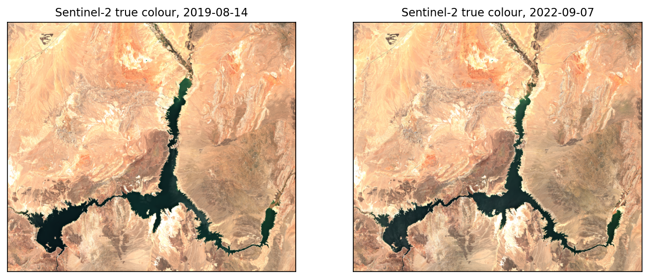

Step 5: water indices and cloud masking

Water reflects green light but absorbs near- and short-wave infrared almost completely. Two normalised-difference indices exploit this:

• NDWI (McFeeters, 1996) = (Green − NIR) / (Green + NIR)
• MNDWI (Xu, 2006) = (Green − SWIR1) / (Green + SWIR1)

In both, open water scores above zero.

with np.errstate(invalid="ignore", divide="ignore"):
    ndwi = (green - nir) / (green + nir)
    mndwi = (green - swir) / (green + swir)
cloudy = np.isin(scl, CLOUD_CLASSES)
valid = ~np.isnan(ndwi) & ~np.isnan(mndwi) & ~cloudy
water = (mndwi > 0) & valid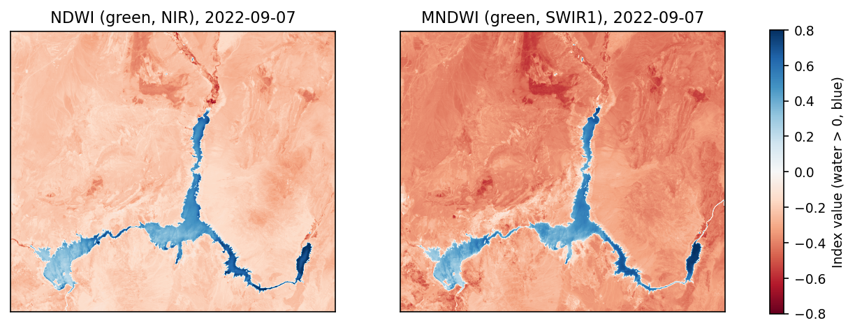

We use MNDWI as the primary water mask and keep NDWI and the SCL’s own water class (6) for comparison:

 year       date  ndwi_km2  water_km2  scl_water_km2  cloud_masked_km2  valid_pct
 2019 2019-08-14     325.7      324.1          379.2               1.7      100.0
 2020 2020-09-02     326.7      323.5          369.4               2.2      100.0
 2021 2021-09-07     299.8      286.5          361.1               2.9       99.9
 2022 2022-09-07     270.1      267.1          349.1               4.1       99.9
 2023 2023-09-07     295.2      289.3          368.0               1.5      100.0
 2024 2024-07-03     290.8      288.9          365.3               2.0      100.0
 2025 2025-09-16     286.1      281.0          357.7               1.0      100.0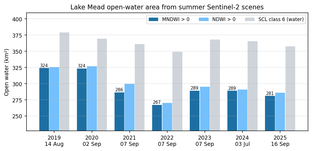

Step 6: map the change

Comparing two boolean masks gives a change map directly:

change = np.zeros((HEIGHT, WIDTH), "uint8")
change[water_masks[first] & water_masks[2022]] = 1          # stayed wet
change[water_masks[first] & ~water_masks[2022]] = 2         # dried out
change[water_masks[2022] & ~water_masks[first]] = 3         # newly wet

water in 2019 but not 2022: 57.6 km²
water in 2022 but not 2019: 0.7 km²
change 2019 -> 2025: -43.1 km²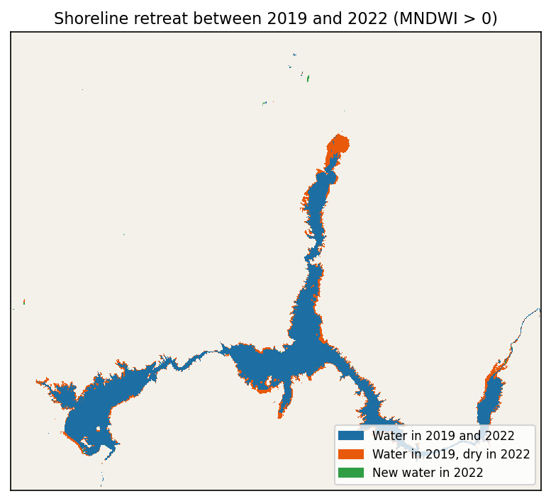

Interpreting the results

• Between summer 2019 and September 2022, Lake Mead’s open-water area fell from 324 km² to 267 km², a loss of about 18 %. Almost 58 km² of former lake bed was exposed, roughly the land area of Manhattan.
• The lake partly recovered in 2023 (289 km²) after the very wet 2022–23 winter, but by September 2025 it had slipped back to 281 km², still 43 km² below 2019.
• Methods disagree on absolute area, but agree on the trend. NDWI is within a few km² of MNDWI. The SCL water class is consistently 50–80 km² higher. It is a general-purpose classifier rather than a tuned water index, and is not designed for precise shoreline mapping. Treat it as a cross-check, not a measurement.
• Area is not volume. The lake’s narrow canyons hold a lot of water in a small surface area. For storage, combine the shoreline with a bathymetric DEM or use the US Bureau of Reclamation’s published elevation-storage data.

Next steps

• Use every clear scene, not one per summer, to build a monthly time series and compare it with the reservoir’s published surface elevation.
• Run at RES = 10 and vectorise the shoreline with rasterio.features.shapes.
• Try the same workflow on another reservoir by changing BBOX and TILES.
• Combine with terrain in Terrain analysis in Python with rasterio and rioxarray.

Data and licences

• Sentinel-2 L2A: contains modified Copernicus Sentinel data 2019–2025, processed by ESA. Accessed as COGs from the AWS Registry of Open Data via Earth Search in October 2026.
• References: McFeeters, S. K. (1996), Int. J. Remote Sensing 17(7); Xu, H. (2006), Int. J. Remote Sensing 27(14).
• Code: lake_mead_ndwi.py, tested with Python 3.8.10, pystac-client 0.7.6 and rasterio 1.3.11.