Terrain analysis in Python: stream, clip and analyse a DEM with rasterio and rioxarray
Read only the pixels you need from a cloud-hosted Copernicus DEM, reproject to British National Grid, derive hillshade, slope and aspect with NumPy, compute zonal statistics and draw an elevation profile — all in one script.
- Level
- Intermediate
- Tested with
- Python 3.8
- Source code
- Download scripts
Key takeaways
- A Cloud Optimised GeoTIFF can be opened over HTTP for a few kilobytes, and rioxarray downloads only the blocks that intersect your area of interest.
- Reproject to a projected CRS in metres before computing slope; use bilinear resampling for elevation and nearest for categorical rasters.
- Hillshade, slope and aspect need only np.gradient and trigonometry; results differ from GDAL and QGIS (Horn kernel) by a fraction of a degree on a 30 m DEM.
- Validate a DEM against published heights: the broad Dark Peak summits came within 2–5 m, typical for a 30 m model.
Before you start
- Comfortable with NumPy arrays and basic GeoPandas (see the GeoPandas getting-started tutorial)
- Python 3.8+ with rasterio, rioxarray and geopandas installed
- An internet connection: the DEM is streamed from AWS Open Data (only the blocks covering the AOI are transferred)
Digital elevation models (DEMs) underpin flood modelling, viewshed analysis, route planning and 3D printing, which is how this site started: see our post on creating a 3D-printed DEM in QGIS. This tutorial reproduces a typical desktop terrain workflow in Python, so you can repeat it for any area by changing one line.
We will work on the Dark Peak in England’s Peak District, from Kinder Scout and Bleaklow east to the Hope Valley, and:
- inspect a Cloud Optimised GeoTIFF (COG) on AWS without downloading it;
- read only our area of interest (AOI) with
rioxarray; - reproject to British National Grid (EPSG:27700) at 30 m;
- compute hillshade, slope and aspect with NumPy;
- compute zonal statistics on a 2 km grid;
- validate the DEM against published summit heights and draw a profile.
All outputs below came from terrain_analysis.py.
The data: Copernicus GLO-30 on AWS
The Copernicus DEM GLO-30 is a free, near-global 30 m surface model derived from the TanDEM-X mission. AWS hosts it as one COG per 1°×1° tile in the public bucket copernicus-dem-30m. The tile names encode the south-west corner, so the tile covering 53–54°N, 2–1°W is:
DEM_URL = ("https://copernicus-dem-30m.s3.amazonaws.com/" "Copernicus_DSM_COG_10_N53_00_W002_00_DEM/Copernicus_DSM_COG_10_N53_00_W002_00_DEM.tif")AOI = (-1.95, 53.30, -1.50, 53.52) # lon/lat bounding box: Dark Peak to the Hope ValleyStep 1: inspect a remote COG
A COG stores its pixels in tiles with internal overviews and puts the metadata at the start of the file. GDAL can therefore read the header and individual tiles with HTTP range requests, so opening a URL with rasterio costs only a few kilobytes:
import rasterio
with rasterio.open(DEM_URL) as src: print("driver:", src.driver) print("size:", src.width, "x", src.height, "| bands:", src.count, "| dtype:", src.dtypes[0]) print("crs:", src.crs) print("resolution (deg):", tuple(round(r, 6) for r in src.res)) print("bounds:", src.bounds) print("overviews:", src.overviews(1)) print("block shape:", src.block_shapes[0])driver: GTiffsize: 2400 x 3600 | bands: 1 | dtype: float32crs: EPSG:4326resolution (deg): (0.000417, 0.000278)bounds: BoundingBox(left=-2.000208333333333, bottom=53.00013888888889, right=-1.0002083333333331, top=54.00013888888889)overviews: [2, 4, 8]block shape: (1024, 1024)The pixels are not square in degrees: 0.000417° × 0.000278°. Above 50° latitude, Copernicus widens the longitude spacing so that pixels stay roughly 30 m wide on the ground. The 1024×1024 blocks are what makes partial reads efficient.
Step 2: read just the AOI with rioxarray
rioxarray wraps rasterio in an xarray.DataArray with labelled x/y coordinates and a .rio accessor for geospatial operations. Opening is lazy: nothing is fetched until we call .load(), and then only the blocks that intersect the clip box are downloaded:
import rioxarray
dem = rioxarray.open_rasterio(DEM_URL, masked=True).squeeze("band", drop=True)dem_aoi = dem.rio.clip_box(*AOI).load()print(dem_aoi)<xarray.DataArray (y: 793, x: 1081)>array([[494.754 , 494.5203 , 494.6352 , ..., 112.59608 , 111.62201 , 110.16745 ], ..., [303.0156 , 300.30637 , 300.6067 , ..., 197.68457 , 196.85437 , 193.29388 ]], dtype=float32)Coordinates: * x (x) float64 -1.95 -1.95 -1.949 -1.949 ... -1.501 -1.5 -1.5 * y (y) float64 53.52 53.52 53.52 53.52 ... 53.3 53.3 53.3 53.3 spatial_ref int32 0Attributes: AREA_OR_POINT: Point scale_factor: 1.0 add_offset: 0.0That is 857,000 pixels instead of the tile’s 8.6 million. masked=True turns the file’s nodata value into NaN, so later statistics ignore it.
Step 3: reproject to British National Grid
Slope maths needs the horizontal and vertical units to match: metres, not degrees. rio.reproject() warps to a projected CRS at an exact resolution. A lat/lon rectangle comes out slightly rotated in BNG, so we trim the result to the largest axis-aligned rectangle that is fully covered by data:
from pyproj import Transformerfrom rasterio.enums import Resampling
dem_bng = dem_aoi.rio.reproject("EPSG:27700", resolution=30, resampling=Resampling.bilinear, nodata=np.nan)
to_bng = Transformer.from_crs("EPSG:4326", "EPSG:27700", always_xy=True)cx, cy = to_bng.transform([AOI[0], AOI[0], AOI[2], AOI[2]], [AOI[1], AOI[3], AOI[1], AOI[3]])dem_bng = dem_bng.rio.clip_box(max(cx[0], cx[1]) + 60, max(cy[0], cy[2]) + 60,                               min(cx[2], cx[3]) - 60, min(cy[1], cy[3]) - 60)
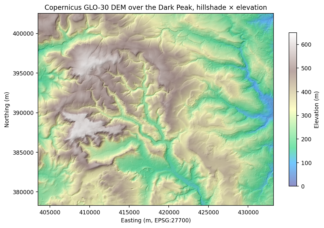
print("crs:", dem_bng.rio.crs, "| shape:", dem_bng.shape, "| res:", dem_bng.rio.resolution())print("elevation min/mean/max (m):", *np.round([float(dem_bng.min()), float(dem_bng.mean()), float(dem_bng.max())], 1))dem_bng.rio.to_raster(OUT / "dem_peak_district_bng.tif", compress="deflate")crs: EPSG:27700 | shape: (809, 991) | res: (30.0, -30.0)elevation min/mean/max (m): 63.8 334.1 634.5Use bilinear (or cubic) resampling for continuous surfaces like elevation, and nearest for categorical rasters such as land cover. The 634.5 m maximum is on the Kinder plateau, whose highest point is published as 636 m. We test that properly in Step 6.
Step 4: hillshade, slope and aspect with NumPy
You do not need a special library for first-derivative terrain attributes. np.gradient gives the rate of change in each direction, and the rest is trigonometry:
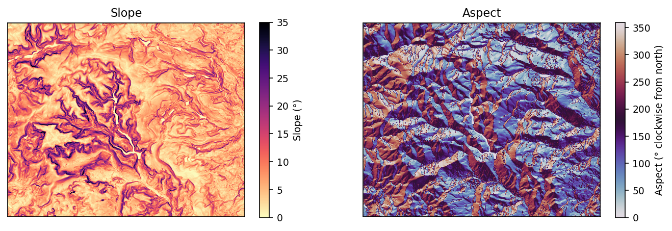
z = dem_bng.values.astype("float64")res = abs(dem_bng.rio.resolution()[0])        # 30 mdz_dy, dz_dx = np.gradient(z, res)            # rows increase southwards...dz_dy = -dz_dy                                # ...so flip to make +y point northslope = np.degrees(np.arctan(np.hypot(dz_dx, dz_dy)))aspect = (np.degrees(np.arctan2(-dz_dx, -dz_dy)) + 360) % 360  # 0 = north-facing, clockwise
ls = LightSource(azdeg=315, altdeg=45)        # sun in the north-west, 45° uphillshade = ls.hillshade(np.nan_to_num(z, nan=np.nanmean(z)), vert_exag=2, dx=res, dy=res)
slope_da = dem_bng.copy(data=slope) wraps the NumPy result back into a georeferenced DataArray, so slope_da.rio.to_raster("slope_deg.tif") writes a GeoTIFF that QGIS opens in the right place.
print(pd.Series(slope[~np.isnan(slope)]).describe(percentiles=[0.5, 0.9, 0.99]).round(2).to_string())count 801719.00mean 8.40std 6.33min 0.0050% 6.5490% 17.5899% 28.96max 50.46Half the area is gentler than 6.5° (the broad moorland plateaus), but the top 1 % is steeper than 29°. These are the gritstone edges and the landslip scarp of Mam Tor.
Step 5: zonal statistics on a 2 km grid
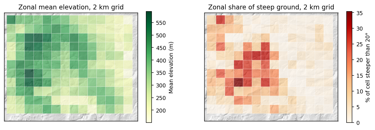
Zonal statistics summarise raster values inside polygons. The fastest pure-Python approach is to rasterise the zones onto the DEM grid once and then use a pandas groupby. No per-polygon loops are needed:
from rasterio.features import rasterizefrom shapely.geometry import box
x0, y0, x1, y1 = dem_bng.rio.bounds()size = 2000cells = [box(x, y, x + size, y + size)         for x in np.arange(np.ceil(x0 / size) * size, x1 - size, size)         for y in np.arange(np.ceil(y0 / size) * size, y1 - size, size)]grid = gpd.GeoDataFrame({"cell_id": range(1, len(cells) + 1)}, geometry=cells, crs="EPSG:27700")
zones = rasterize(zip(grid.geometry, grid.cell_id), out_shape=z.shape, transform=dem_bng.rio.transform(), fill=0, dtype="int32")df = pd.DataFrame({"cell_id": zones.ravel(), "elev": z.ravel(), "slope": slope.ravel()})df = df[(df.cell_id > 0) & df.elev.notna()]stats = df.groupby("cell_id").agg(elev_mean=("elev", "mean"), elev_max=("elev", "max"), slope_mean=("slope", "mean"), steep_pct=("slope", lambda s: (s > 20).mean() * 100), n_pixels=("elev", "size"))grid = grid.merge(stats.reset_index(), on="cell_id")print(grid.nlargest(5, "slope_mean").drop(columns="geometry").round(1).to_string(index=False)) cell_id elev_mean elev_max slope_mean steep_pct n_pixels 49 394.2 579.8 15.4 26.5 4422 37 499.5 625.8 14.8 35.3 4422 22 381.6 513.3 14.8 27.8 4422 62 379.3 480.2 14.6 29.6 4422 16 460.2 622.9 14.5 23.3 4422Each 2 km cell should contain (2000/30)² ≈ 4,444 pixels; the counts of 4,422 and 4,489 reflect where cell edges fall between pixel centres. Cell 37 has over a third of its ground steeper than 20°: it contains the Kinder edges.
Step 6: validate against published summit heights
Never trust a DEM blindly. Here we compare it with published spot heights for five summits, sampling both the nearest pixel and the highest pixel within 300 m, to allow for small errors in the summit coordinates:
for geom in summits.geometry: point_vals.append(float(dem_bng.sel(x=geom.x, y=geom.y, method="nearest"))) window = dem_bng.rio.clip([geom.buffer(300)], crs="EPSG:27700") max_vals.append(float(window.max())) name published_m dem_at_point dem_max_300m Kinder Scout 636 631.9 634.4 Bleaklow 633 628.1 629.5 Mam Tor 517 511.3 512.6 Win Hill 462 445.0 454.2Stanage Edge (High Neb) 458 428.5 439.2The broad summits (Kinder, Bleaklow, Mam Tor) come within 2–5 m of their published heights, which is typical for a 30 m DEM. Each pixel is an average over roughly 900 m², which shaves the top off any peak. GLO-30 heights are also relative to the EGM2008 geoid rather than Ordnance Datum Newlyn, so expect small systematic differences from OS heights. Win Hill’s small rocky top and the narrow crest of Stanage Edge lose much more, and our High Neb coordinate is approximate. Small, sharp features are where coarse DEMs fail. Bear that in mind before calculating viewsheds or line-of-sight from a summit.
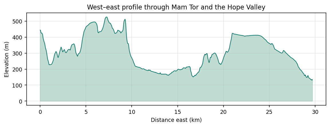
Finally, an east–west profile through Mam Tor uses xarray’s label-based selection: dem_bng.sel(y=<northing>, method="nearest") returns one row of the DEM.
Summary
| Task | Tool |
|---|---|
| Inspect a remote raster cheaply | rasterio.open(url) on a COG |
| Lazy, labelled raster arrays | rioxarray.open_rasterio(..., masked=True) |
| Clip / reproject / write | .rio.clip_box(), .rio.clip(), .rio.reproject(), .rio.to_raster() |
| Slope, aspect, hillshade | np.gradient, matplotlib.colors.LightSource |
| Zonal statistics | rasterio.features.rasterize + pandas groupby |
Next steps
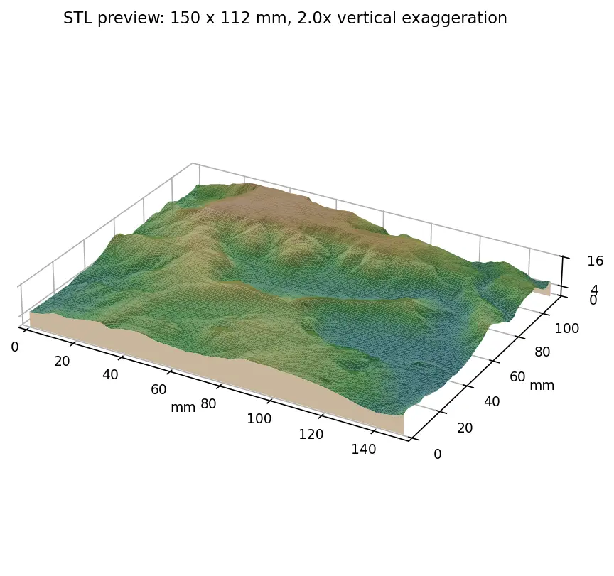
- Turn this DEM into a physical model in From DEM to 3D-printable STL with Python.
- Swap in a 1 m Environment Agency LiDAR DTM (UK data sources) and watch the summit errors shrink.
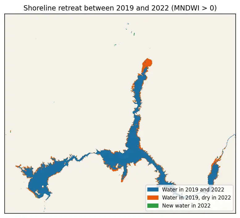
- Combine terrain with satellite imagery in Measuring Lake Mead’s shrinking shoreline with Sentinel-2 and STAC.
Data and licences
- Copernicus DEM GLO-30: © DLR e.V. 2010–2014 and © Airbus Defence and Space GmbH 2014–2018, provided under COPERNICUS by the European Union and ESA; all rights reserved. Free to use under the Copernicus DEM licence. Accessed via the AWS Open Data registry in October 2026.
- Published summit heights are taken from Ordnance Survey mapping. High Neb’s coordinates are approximate.
- Code:
terrain_analysis.py, tested with Python 3.8.10, rasterio 1.3.11 and rioxarray 0.13.4.
Key terms
- COG
- A Cloud Optimised GeoTIFF stores tiles and overviews so clients can read parts of the file with HTTP range requests.
- Hillshade
- A greyscale rendering of terrain lit from a chosen sun angle, used to show relief.
- Slope and aspect
- Slope is the steepness of the terrain in degrees; aspect is the compass direction a slope faces.
- Zonal statistics
- Summaries (mean, maximum, share above a threshold) of raster values inside each polygon zone.
Data for this tutorial
- Copernicus DEM (GLO-30 / GLO-90) · Global 30 m elevation, free with attribution
- GIS data sources for the United Kingdom
Licences and formats for each source are listed in the GIS data sources catalogue.