Creating a 3D printed digital elevation model can be achieved using QGIS and the DEMto3D plugin. This tutorial demonstrates the creation of a 3D STL file that can be printed using a 3D printer.
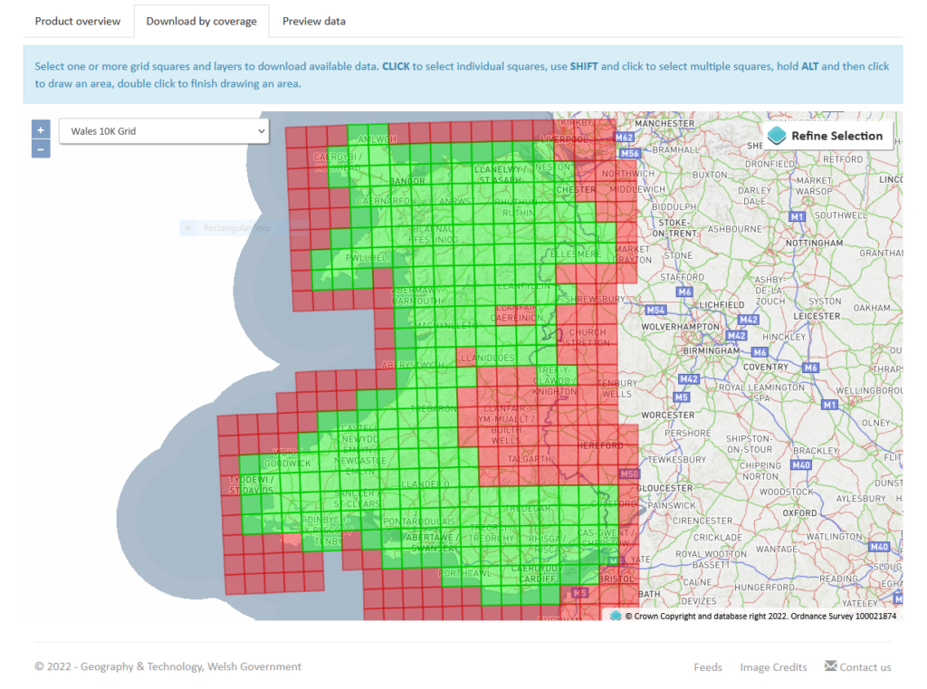
This example uses digital elevation data obtained from the Lle Geo-Portal that covers nearly all of the area of Wales, United Kingdom.
Software used:
QGIS Version 3.6.3-Noosa (https://qgis.org/en/site/forusers/download.html)
Lle Geo-Portal (http://lle.gov.wales/GridProducts#data=LidarCompositeDataset)
Screenshot of the Lle Geo-Portal website.
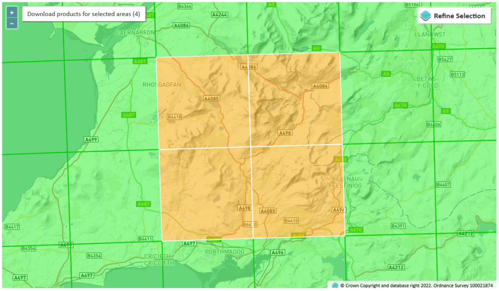
Elevation data at 1 metre resolution has been obtained from the Lle Geo-Portal for this tutorial. A total of four grid squares have been downloaded and the area of interest will be refined using QGIS in a later step. The image below shows the four grid squares chosen.
The grid squares chosen to download were:
LiDAR Composite Dataset – DTM – 1m – ASC – SH55
LiDAR Composite Dataset – DTM – 1m – ASC – SH65
LiDAR Composite Dataset – DTM – 1m – ASC – SH64
LiDAR Composite Dataset – DTM – 1m – ASC – SH54
Image displaying the grid squares chosen for the tutorial.
After creating a new project in QGIS, import the elevation data using the Layer -> Add Layer -> Add Raster Layer menu option. The data is downloaded in the ZIP file format containing multiple ASC files that can be imported directly into QGIS. ASC files essentially contains lists of cell values, which in this case are elevation values in metres.
Due to the number of individual files and for ease of visualisation, each of the individual files will be merged to create a raster mosaic. The contents of each ZIP file be merged initially, then finally the four resulting rasters will be merged together to form a single raster mosaic.
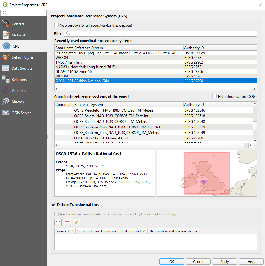
Data downloaded from the Lle Geo-Portal is projected in OSGB 1936 / British National Grid and this projection should be selected in the project properties, as shown below.
Screenshot showing the QGIS project projection properties.
Using the GDAL -> Raster Miscellaneous -> Merge tool available in the Processing Toolbox, merge the individual rasters to create a single raster.
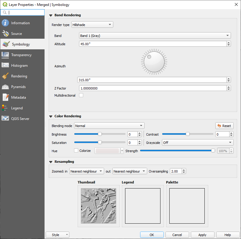
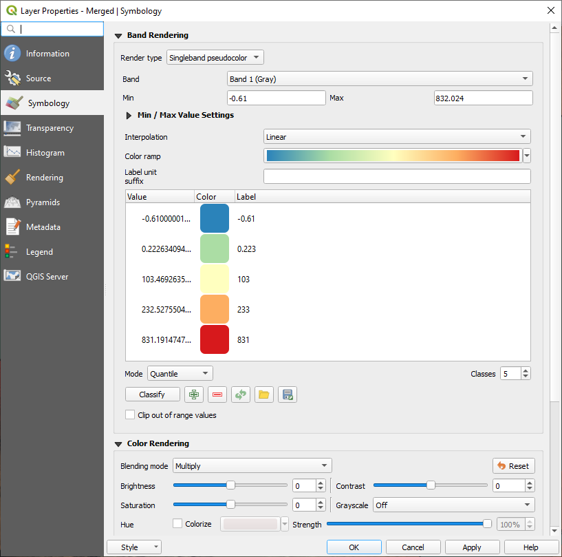
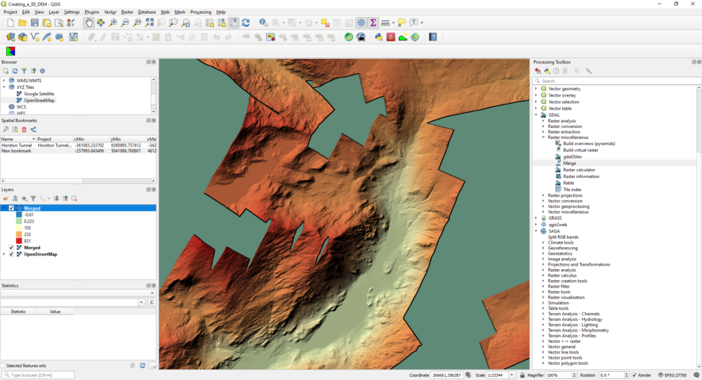
The next step is optional and is used to visualise the elevation. Duplicate the elevation layer and set the layer symbology to Hillshade on the first layer, as shown in the image below. On the second layer, set the layer symbology to Singleband Psuedocolor, making sure to set the Blending Mode to Multiply in the Color Rendering options panel.
Once the symbology has been applied, the digital elevation layers should appear as below.
Screenshot showing digital elevation layers with symbology applied.
The next step is clip the area of interest from the raster, ensuring there are no gaps contained within the elevation data as this would cause issues with creating the STL in later steps.
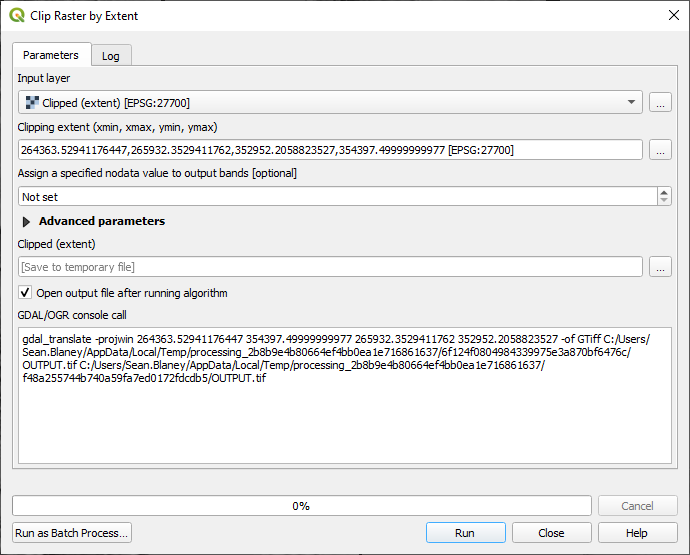
Using the GDAL -> Raster Extraction -> Clip Raster by Extent tool in the Processing Toolbox to clip an area of interest as shown in the screen of the ‘Clip Raster by Extent’ dialog box shown below.
Screenshot of the Clip Raster by Extent dialog.
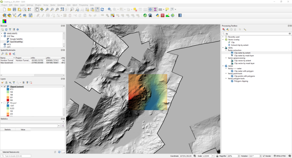
Screenshot showing the clipped elevation layer.
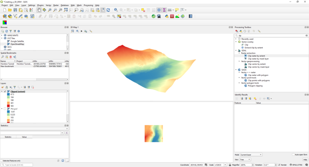
The resulting clipped layer is visualised in 3D within the 3D Map View in the screenshot below, using the settings shown in the screenshot of the 3D Configuration settings.
Visualisation of the digital elevation data in 3D.
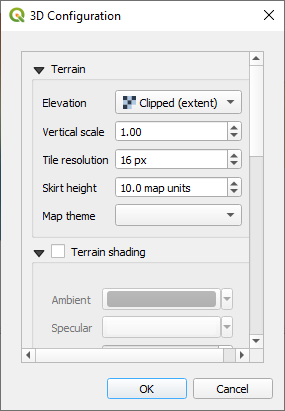
Screenshot of the 3D configuration settings.
Once an area of interest has been clipped from the full raster containing the elevation data, open a 3D map view from the View -> New 3D Map View menu selection.
Isolate the clipped layer and set the terrain elevation in the 3D Map view settings dialog to the clipped extent.
Finally, create the 3D printable STL file using the DEMto3D QGIS plugin, available from the Raster -> DEMto3D -> DEM 3D printing menu option.
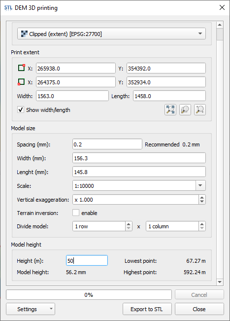
Using the options shown in the DEMto3D settings dialog below, configure the properties of the resulting STL file according to your desired printing properties including final printed model dimensions.
Screenshot of the DEMto3D settings dialog.
Once the desired properties have been chosen, simply click ‘Export to STL’ to create an STL suitable for printing.
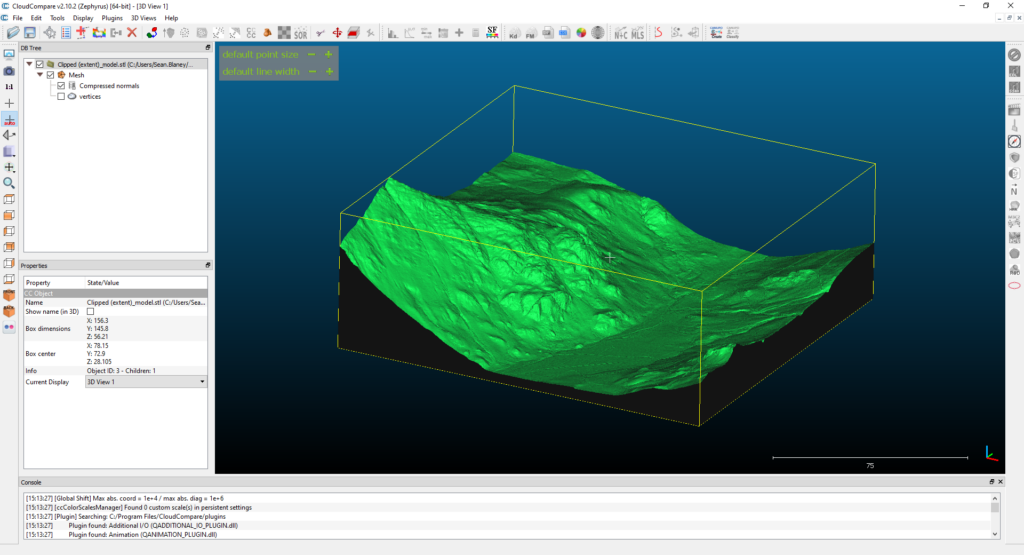
Finally, results can be visualised in your favourite 3D printing software or alternatively loaded in CloudCompare for quick visualisation and to check the quality of the STL file output.
Visualisation of the final STL file using CloudCompare.
We use cookies on our website to give you the most relevant experience by remembering your preferences and repeat visits. By clicking “Accept All”, you consent to the use of ALL the cookies. However, you may visit "Cookie Settings" to provide a controlled consent.
This website uses cookies to improve your experience while you navigate through the website. Out of these, the cookies that are categorized as necessary are stored on your browser as they are essential for the working of basic functionalities of the website. We also use third-party cookies that help us analyze and understand how you use this website. These cookies will be stored in your browser only with your consent. You also have the option to opt-out of these cookies. But opting out of some of these cookies may affect your browsing experience.
Necessary cookies are absolutely essential for the website to function properly. These cookies ensure basic functionalities and security features of the website, anonymously.
Cookie
Duration
Description
cookielawinfo-checkbox-analytics
11 months
This cookie is set by GDPR Cookie Consent plugin. The cookie is used to store the user consent for the cookies in the category "Analytics".
cookielawinfo-checkbox-functional
11 months
The cookie is set by GDPR cookie consent to record the user consent for the cookies in the category "Functional".
cookielawinfo-checkbox-necessary
11 months
This cookie is set by GDPR Cookie Consent plugin. The cookies is used to store the user consent for the cookies in the category "Necessary".
cookielawinfo-checkbox-others
11 months
This cookie is set by GDPR Cookie Consent plugin. The cookie is used to store the user consent for the cookies in the category "Other.
cookielawinfo-checkbox-performance
11 months
This cookie is set by GDPR Cookie Consent plugin. The cookie is used to store the user consent for the cookies in the category "Performance".
viewed_cookie_policy
11 months
The cookie is set by the GDPR Cookie Consent plugin and is used to store whether or not user has consented to the use of cookies. It does not store any personal data.
Functional cookies help to perform certain functionalities like sharing the content of the website on social media platforms, collect feedbacks, and other third-party features.
Performance cookies are used to understand and analyze the key performance indexes of the website which helps in delivering a better user experience for the visitors.
Analytical cookies are used to understand how visitors interact with the website. These cookies help provide information on metrics the number of visitors, bounce rate, traffic source, etc.
Advertisement cookies are used to provide visitors with relevant ads and marketing campaigns. These cookies track visitors across websites and collect information to provide customized ads.