Fast vector geoprocessing in Python: spatial indexes, overlays and modern file formats

GeoPandas code that works on a 500-row sample often grinds to a halt on real data. The cause is almost always the same: a Python loop where a vectorised, spatially indexed operation should be. Since Shapely 2.0, every geometry operation runs on whole NumPy arrays in C (GEOS), and GeoPandas uses it automatically.

This tutorial measures the difference rather than just asserting it. We will:

1. generate a realistic dataset: about 200,000 “incident” points clustered around British towns, and a 5 km analysis grid;
2. assign points to grid cells three ways (naive loop, STRtree, sjoin) and time each;
3. look at the speed/accuracy trade-off for buffers;
4. run an overlay and two flavours of dissolve;
5. write and read the same data as Shapefile, GeoPackage, FlatGeobuf and GeoParquet.

Every timing below comes from a single run of vector_performance.py on a Windows 11 laptop. Your absolute numbers will differ; the ratios are what matter.

=== versions ===
geopandas 0.13.2 | shapely 2.0.7 | GEOS 3.11.4

Step 1: build a test dataset

Synthetic data lets you control the size and still get a realistic spatial distribution. We take the British towns from Natural Earth’s 1:10m populated places and scatter 250,000 points around them, weighted by population with an 8 km Gaussian spread. A quarter of the points are spread uniformly as background noise. Everything is in British National Grid (EPSG:27700), so distances are in metres.

countries = gpd.read_file(fetch("ne_50m_admin_0_countries.zip"), engine="pyogrio")
uk = countries.loc[countries.ADM0_A3 == "GBR", ["geometry"]].to_crs(27700)
gb = uk.explode(index_parts=False).reset_index(drop=True)  # parts share one label until reset
gb = gb.loc[[gb.area.idxmax()]]  # the island of Great Britain only
places = gpd.read_file(fetch("ne_10m_populated_places.zip"), engine="pyogrio")
towns = places.loc[places.ADM0_A3 == "GBR"].to_crs(27700).clip(gb)

N = 250_000
rng = np.random.default_rng(42)
w = towns.POP_MAX.to_numpy(float)
centre = rng.choice(len(towns), size=N, p=w / w.sum())
xy = np.column_stack([towns.geometry.x.to_numpy()[centre], towns.geometry.y.to_numpy()[centre]])
xy += rng.normal(scale=8_000, size=(N, 2))
noise = rng.random(N) < 0.25  # a quarter of points spread uniformly
minx, miny, maxx, maxy = gb.total_bounds
xy[noise] = np.column_stack([rng.uniform(minx, maxx, noise.sum()), rng.uniform(miny, maxy, noise.sum())])
points = gpd.GeoDataFrame(
    {"id": np.arange(N), "category": rng.choice(["burglary", "vehicle", "criminal damage", "theft"], N),
     "value": rng.gamma(2.0, 50.0, N).round(2)},
    geometry=gpd.points_from_xy(xy[:, 0], xy[:, 1]), crs=27700)
points = points[points.intersects(gb.geometry.iloc[0])].reset_index(drop=True)

There are two vectorised tricks already here. gpd.points_from_xy builds all the points in one call. points.intersects(polygon) tests all 250,000 points against Great Britain at once and keeps only those on land.

The grid is also built without a loop. shapely.box accepts arrays of coordinates:

cell = 5_000
gx, gy = np.meshgrid(np.arange(minx // cell * cell, maxx, cell), np.arange(miny // cell * cell, maxy, cell))
grid = gpd.GeoDataFrame(geometry=shapely.box(gx.ravel(), gy.ravel(), gx.ravel() + cell, gy.ravel() + cell),
                        crs=27700)
grid = grid[grid.intersects(gb.geometry.iloc[0])].reset_index(drop=True)
grid["cell_id"] = np.arange(len(grid))
grid["region"] = ((grid.geometry.bounds.minx // 100_000).astype(int).astype(str) + "-"
                  + (grid.geometry.bounds.miny // 100_000).astype(int).astype(str))

=== test data ===
towns used as cluster centres: 48
points: 202,062  grid cells: 9,255  regions: 43
   id         category   value                       geometry
0   0         burglary  134.29  POINT (330043.351 657750.024)
1   1  criminal damage  101.07  POINT (389617.801 296168.657)
2   2         burglary  146.95  POINT (438262.667 513892.769)
3   3          vehicle   35.88  POINT (350664.759 393165.710)
4   4         burglary   85.89  POINT (203502.102 871590.272)

Of the 250,000 generated points, 202,062 fall on Great Britain; the rest fell offshore. The region column is a 100 km grid-square code that we will dissolve on later.

Step 2: point-in-polygon, three ways

The task is to find which of the 9,255 cells contains each point.

The naive loop

This is the version most people write first: for each point, test every polygon.

sample = points.iloc[:2_000]
naive = []
for pt in sample.geometry:
    hit = grid.index[grid.contains(pt)]
    naive.append(hit[0] if len(hit) else -1)

grid.contains(pt) is itself vectorised, but it still performs 9,255 full geometry tests per point. We only time 2,000 points and extrapolate the rest.

A Shapely STRtree

An STRtree (Sort-Tile-Recursive R-tree) stores each polygon’s bounding box in a balanced tree. A query first finds the handful of candidate boxes that overlap the point, then runs the exact predicate on those candidates only. Shapely 2 can query an entire array of geometries at once and returns pairs of indices:

tree = shapely.STRtree(grid.geometry.values.data)
pt_idx, poly_idx = tree.query(points.geometry.values.data, predicate="within")

GeoPandas sjoin

sjoin builds the same STRtree internally (grid.sindex) and returns a joined GeoDataFrame:

joined = gpd.sjoin(points, grid[["cell_id", "geometry"]], how="inner", predicate="within")

=== point-in-polygon ===
naive loop (2,000 points)                     0.393 s
  -> extrapolated to all points                39.7 s
STRtree.query, all points                     0.130 s
gpd.sjoin, all points                         0.246 s
matched 202,062 of 202,062 points; all three methods agree
sjoin speed-up over naive loop: ~161x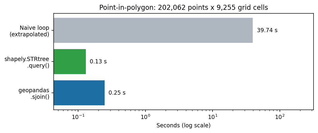

The script asserts that all three methods return the same assignments, so the speed-up costs nothing in correctness. Counting points per cell is then an ordinary pandas groupby:

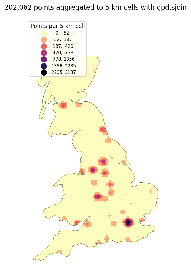
counts = joined.groupby("cell_id").size().rename("n_points")
grid = grid.join(counts, on="cell_id").fillna({"n_points": 0}).astype({"n_points": int})

      cell_id region  n_points
1532     1532    5-1      3137
1593     1593    5-1      3057
1531     1531    5-1      2935
1592     1592    5-1      2873
1533     1533    5-1      2235

The five busiest cells are all in 100 km square 5-1 (eastings 500–600 km, northings 100–200 km), which is central London.

Step 3: buffers and quad_segs

A buffer around a point is a polygon that approximates a circle. The resolution argument (called quad_segs in Shapely) sets how many segments make up each quarter circle:

subset = points.iloc[:50_000]
b16 = subset.buffer(500)                 # default: 16 segments per quarter circle
b4 = subset.buffer(500, resolution=4)

=== buffers ===
buffer 500 m, quad_segs=16 (default)          0.442 s
buffer 500 m, quad_segs=4                     0.318 s
vertices per buffer: 65 vs 17; area error of quad_segs=4: 2.55%

Creating the buffers is only about 30 % faster, but each polygon has a quarter of the vertices. Every downstream overlay, union and file write gets cheaper as a result. The coarse buffer under-estimates the circle’s area by 2.55 %. Whether that matters depends on your analysis. For a “within roughly 500 m” screen it rarely does.

Step 4: unions and overlays

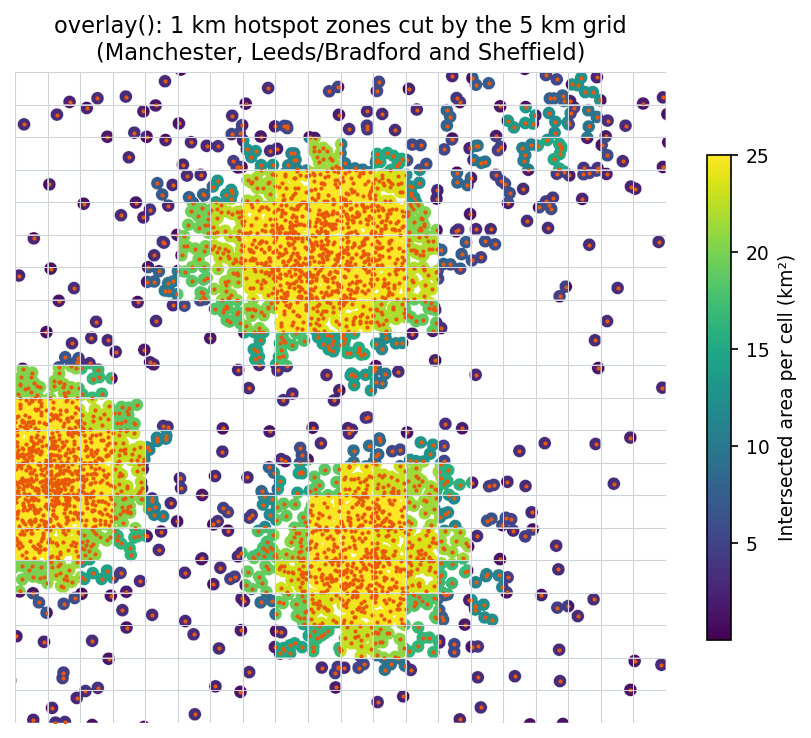
Next, we build “hotspot zones” by buffering 20,000 burglary points by 1 km and merging the overlaps. Then we cut those zones by the grid with overlay:

burglary = points[points.category == "burglary"].iloc[:20_000]
zones = gpd.GeoDataFrame(geometry=[burglary.buffer(1_000, resolution=8).unary_union], crs=27700)
zones = zones.explode(index_parts=False).reset_index(drop=True)

inter = gpd.overlay(grid[["cell_id", "region", "geometry"]], zones, how="intersection")
inter["area_km2"] = inter.area / 1e6
cover = inter.groupby("cell_id").area_km2.sum()

=== overlay ===
buffer + unary_union (20,000 x 1 km)          1.761 s
merged into 3,585 hotspot polygons
overlay(grid, zones, 'intersection')          0.470 s
8,373 intersection pieces; 659 cells are more than half covered

unary_union is the expensive step: 20,000 overlapping circles have to be noded together. overlay is fast because it also uses a spatial index, so it only intersects cell–zone pairs whose bounding boxes overlap.

Step 5: dissolve, and a faster union for coverages

dissolve groups rows and unions their geometries. For polygons that tile without overlapping, such as our grid, Shapely 2 offers coverage_union_all. It assumes the input is a valid coverage (no overlaps), so it can simply drop the shared edges:

regions = grid.dissolve(by="region", aggfunc={"n_points": "sum"})
cov = {r: shapely.coverage_union_all(g.geometry.values.data) for r, g in grid.groupby("region")}

=== dissolve ===
dissolve(by='region')  [unary_union]          0.197 s
coverage_union_all per region                 0.035 s
43 regions; max area difference between methods: 0.000000 m²

The two methods give identical results, but coverage_union_all was more than 5x faster here.

Step 6: choosing a file format

Finally, we write the 202,062 points to four formats. For each one we time a full write, a full read, and a bounding-box read of a 30 × 30 km window around Manchester and Sheffield. The bounding-box read is the operation a web map or a tiled analysis performs.

query_box = box(420_000, 420_000, 450_000, 450_000)
points.to_file("points.gpkg", driver="GPKG", engine="pyogrio")   # .shp / .fgb are the same
points.to_parquet("points.parquet")

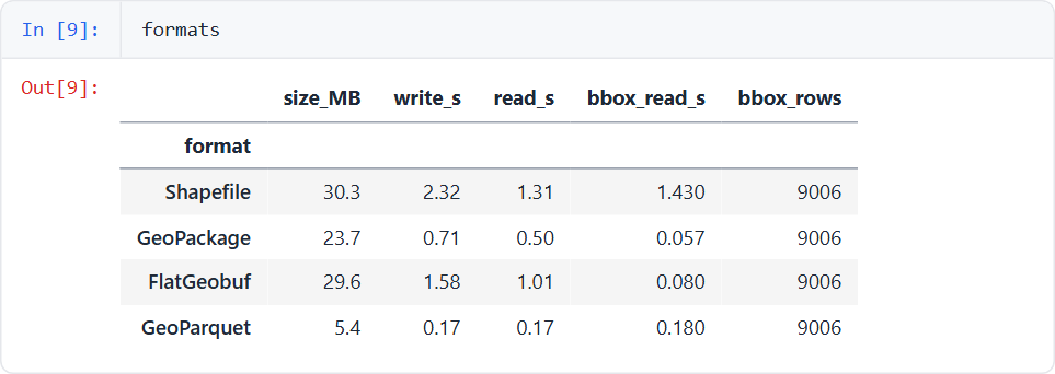
sub = gpd.read_file("points.gpkg", engine="pyogrio", bbox=query_box.bounds)
sub = gpd.read_parquet("points.parquet"); sub = sub[sub.intersects(query_box)]  # gpd 0.13

=== file formats ===
            size_MB  write_s  read_s  bbox_read_s  bbox_rows
format
Shapefile      30.3     2.32    1.31        1.430       9006
GeoPackage     23.7     0.71    0.50        0.057       9006
FlatGeobuf     29.6     1.58    1.01        0.080       9006
GeoParquet      5.4     0.17    0.17        0.180       9006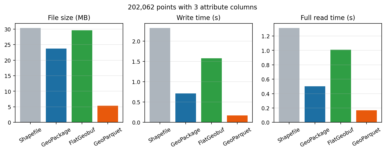

The results tell a clear story:

• GeoParquet is columnar and compressed. It is about 5.5x smaller than a Shapefile and 7–8x faster to read in full. It is the best choice for analysis pipelines and cloud storage. With geopandas 0.13 a bbox read means reading everything and then filtering. geopandas ≥ 1.0 adds read_parquet(bbox=...), which uses GeoParquet 1.1 bbox covering columns to skip row groups.
• GeoPackage has a built-in R-tree, which makes it the fastest at bbox queries here (0.057 s). It is a single file, is the OGC standard and QGIS handles it well. It is the best desktop and interchange format.
• FlatGeobuf also has a spatial index (0.080 s bbox read) and is designed to be streamed over HTTP: a web client can fetch only the bytes for one area from a static file. It is not compact, though.
• Shapefile came last on every measure, and also has a 10-character field-name limit, a 2 GB size limit and needs at least three sidecar files. Use it only when a recipient insists.

Summary: a performance checklist

1. Never loop over geometries in Python. Look for the vectorised method on the GeoSeries, or a shapely.* array function.
2. Use a spatial index for any “which A is in or near which B” question: sjoin, sjoin_nearest, sindex.query or STRtree.
3. Work in a projected CRS with metre units before buffering or measuring.
4. Reduce vertices early: coarser buffers, simplify(), or clipping to your study area.
5. Use coverage_union_all to dissolve clean, non-overlapping tilings.
6. Store intermediates as GeoParquet; deliver as GeoPackage, or FlatGeobuf for the web.

Next steps

• Apply these techniques to real data: GIS data sources for the UK lists open crime, boundary and address datasets.
• For data that doesn’t fit in memory, look at dask-geopandas (the same API, partitioned) or DuckDB’s spatial extension, which can query GeoParquet with SQL.
• Turn a result into an interactive map with Folium.

Data and licences

• Natural Earth 1:50m countries and 1:10m populated places: public domain, naturalearthdata.com.
• The incident points are synthetic, generated by the script with a fixed random seed (42). They are not real crime data.
• Code: vector_performance.py, tested with Python 3.8.10, geopandas 0.13.2, shapely 2.0.7, pyogrio 0.9.0 and pyarrow 17.0.0.