Interactive web maps from Python with Folium and GeoPandas .explore()
Turn GeoDataFrames into shareable Leaflet web maps: a one-line choropleth with .explore(), then a hand-built Folium map with custom styling, tooltips, clustered markers, switchable basemaps and plugins — saved as a single HTML file.
- Level
- Beginner
- Tested with
- Python 3.8
- Source code
- Download scripts
Key takeaways
- GeoDataFrame.explore() makes an interactive, classified choropleth with tooltips and a legend in one line.
- Folium writes a self-contained Leaflet HTML file; the GeoJSON is embedded, so simplify geometries and keep only the columns you need.
- Folium and Leaflet expect [lat, lon], while Shapely and GeoJSON use (lon, lat). Swapping them is the most common Folium bug.
- Use basemaps that need no API key, and always pass attr= for custom tile URLs.
Before you start
- Basic GeoPandas (see the GeoPandas getting-started tutorial)
- Python 3.8+ with geopandas, folium, mapclassify and matplotlib
- A modern web browser to open the generated HTML
A static PNG is perfect for a report, but colleagues and clients increasingly expect to pan, zoom and click. Folium writes Leaflet.js maps from Python. The output is a single self-contained HTML file you can email, drop on a web server or embed in a page, as we do below. No GIS server or JavaScript knowledge is required.
In this tutorial you will:
- make an interactive choropleth in one line with
GeoDataFrame.explore(); - build a richer map with the Folium API: switchable basemaps, a styled choropleth with hover highlight and tooltips, clustered markers with popups, an optional layer and plugins (fullscreen, minimap and measure);
- learn the practical tricks for keeping the HTML small and fast.
The code is in folium_maps.py. The screenshots were taken from its output with Playwright, and the live map near the end is the exact file the script wrote.
Step 1: prepare the data
We use Natural Earth 1:50m countries and populated places. We compute area in an equal-area CRS (EPSG:3035, ETRS89 LAEA Europe), as covered in the GeoPandas tutorial:
countries = gpd.read_file(fetch("ne_50m_admin_0_countries.zip"))countries = countries[["NAME", "CONTINENT", "POP_EST", "GDP_MD", "geometry"]].rename(    columns={"NAME": "name", "CONTINENT": "continent", "POP_EST": "population", "GDP_MD": "gdp_musd"})europe = countries[countries["continent"] == "Europe"].copy()europe["area_km2"] = europe.to_crs("EPSG:3035").area / 1e6europe["density"] = (europe["population"] / europe["area_km2"]).round(1)europe["gdp_per_capita"] = (europe["gdp_musd"] * 1e6 / europe["population"]).round(0)europe = europe[europe["population"] > 0]
places = gpd.read_file(fetch("ne_50m_populated_places.zip"))[["NAME", "ADM0NAME", "POP_MAX", "geometry"]]places = places.rename(columns={"NAME": "city", "ADM0NAME": "country", "POP_MAX": "population"})eu_places = gpd.sjoin(places, europe[["geometry"]], predicate="within").drop(columns="index_right")50 European countries; 209 populated places name population area_km2 density Monaco 38964.0 12.0 3133.0 Malta 502653.0 274.0 1836.0Guernsey 62792.0 48.0 1302.0 Vatican 825.0 1.0 1166.0 Jersey 107800.0 127.0 851.0Before mapping, there are two preparation steps:
# Clip to a European window: Russia crosses the antimeridian and would otherwise# draw a band across the whole map.europe = europe.clip((-25, 34, 50, 72))# Simplify geometries (~1 km) to keep the HTML small: the browser draws every vertex.europe["geometry"] = europe.to_crs("EPSG:3035").simplify(1000).to_crs("EPSG:4326")Folium embeds the GeoJSON inside the HTML file, so every vertex costs bytes and rendering time. Simplifying to a 1 km tolerance in a metric CRS makes no visible difference at continental zoom levels.
Step 2: the one-liner, .explore()
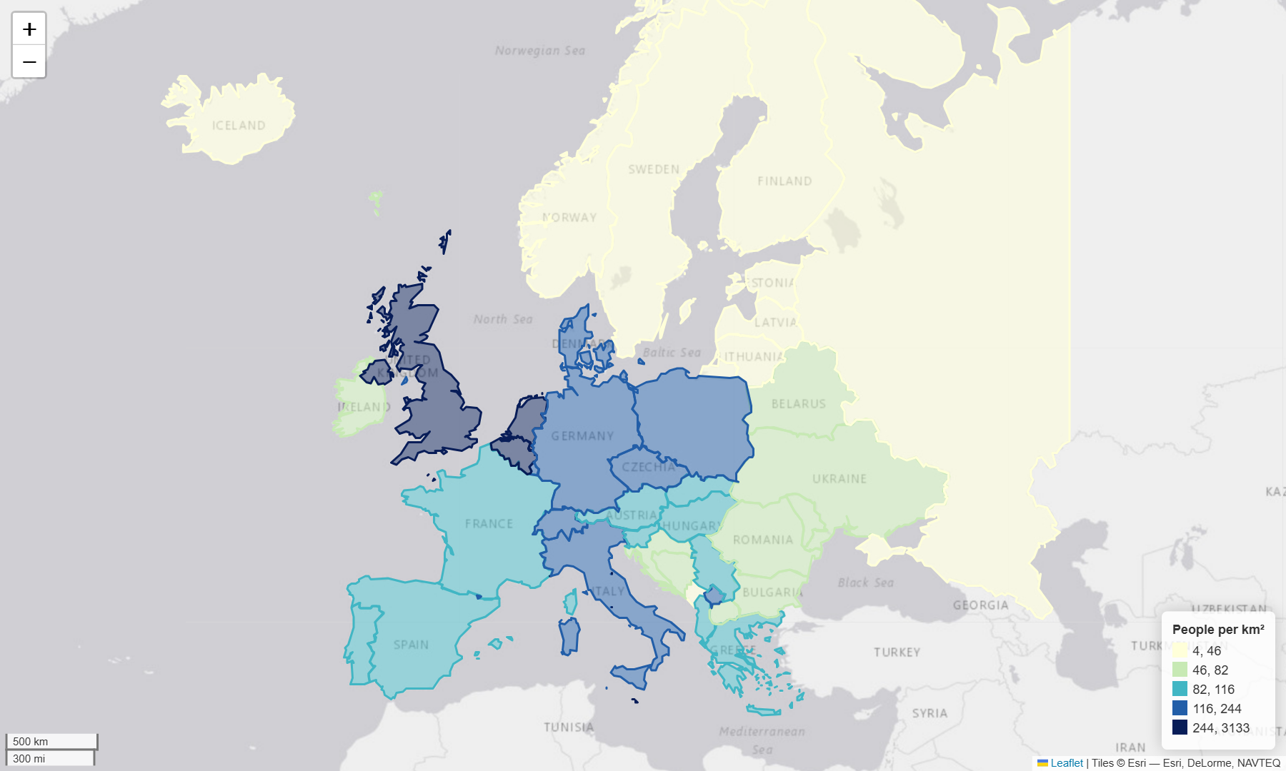
GeoPandas has Folium built in. explore() handles classification (via mapclassify), the colour map, tooltips and the legend:
ESRI_GRAY = "https://server.arcgisonline.com/ArcGIS/rest/services/Canvas/World_Light_Gray_Base/MapServer/tile/{z}/{y}/{x}"ESRI_GRAY_ATTR = "Tiles © Esri — Esri, DeLorme, NAVTEQ"
m1 = europe.explore(column="density", scheme="Quantiles", k=5, cmap="YlGnBu",                    tooltip=["name", "population", "density"],                    legend_kwds={"caption": "People per km²", "colorbar": False, "fmt": "{:.0f}"},                    tiles=ESRI_GRAY, attr=ESRI_GRAY_ATTR, location=[54, 15], zoom_start=4)m1.save("output/explore_density.html")
In a Jupyter notebook, just put m1 on the last line of a cell to display the map inline.
Step 3: a hand-crafted Folium map
For full control, build the map yourself. Start with an empty map and add several base layers. Only one base layer is shown at a time, and the layer control lets users switch between them:
import branca.colormap as cmimport foliumfrom folium import plugins
m = folium.Map(location=[54, 12], zoom_start=4, tiles=None, control_scale=True)folium.TileLayer("OpenStreetMap", name="OpenStreetMap").add_to(m)folium.TileLayer(ESRI_GRAY, attr=ESRI_GRAY_ATTR, name="Light grey (Esri)").add_to(m)folium.TileLayer(    tiles="https://server.arcgisonline.com/ArcGIS/rest/services/World_Imagery/MapServer/tile/{z}/{y}/{x}",    attr="Tiles © Esri — Source: Esri, Maxar, Earthstar Geographics, and the GIS User Community",    name="Esri World Imagery").add_to(m)
A styled choropleth with tooltips
folium.GeoJson takes a style_function that is called for each feature. We use a branca colour map, clipped to the 5th–95th percentile so that outliers don’t wash out the scale, and a highlight_function for hover feedback:
colormap = cm.LinearColormap(["#f7fcf0", "#7bccc4", "#0868ac"],                             vmin=float(europe.gdp_per_capita.quantile(0.05)),                             vmax=float(europe.gdp_per_capita.quantile(0.95)),                             caption="GDP per capita (USD, Natural Earth estimates)")
folium.GeoJson(    europe[["name", "population", "density", "gdp_per_capita", "geometry"]],    name="GDP per capita",    style_function=lambda f: {"fillColor": colormap(f["properties"]["gdp_per_capita"]),                              "color": "#475569", "weight": 0.6, "fillOpacity": 0.7},    highlight_function=lambda f: {"weight": 2.5, "color": "#e8590c", "fillOpacity": 0.85},    tooltip=folium.GeoJsonTooltip(fields=["name", "gdp_per_capita", "density"],                                  aliases=["Country", "GDP per capita (USD)", "People per km²"],                                  localize=True, sticky=True),).add_to(m)colormap.add_to(m)
Select only the columns you need before passing a GeoDataFrame to GeoJson. Every attribute is serialised into the HTML file.
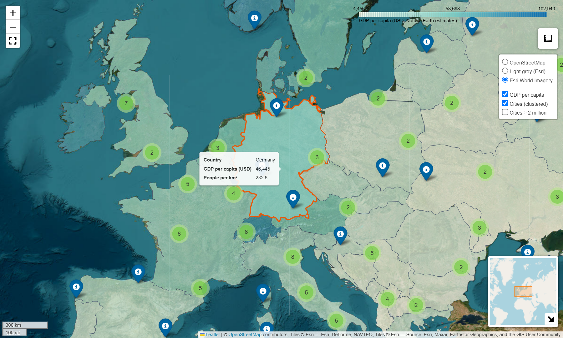
Clustered markers with popups
Plotting 209 individual markers clutters a continental map. MarkerCluster groups nearby markers into numbered bubbles that split apart as you zoom in:
cluster = plugins.MarkerCluster(name="Cities (clustered)").add_to(m)for _, r in eu_places.iterrows(): folium.Marker( location=[r.geometry.y, r.geometry.x], # Folium wants [lat, lon]! tooltip=r["city"], popup=folium.Popup(f"<b>{r['city']}</b><br>{r['country']}<br>Population: {r['population']:,}", max_width=220), icon=folium.Icon(color="darkblue", icon="info-sign"), ).add_to(cluster)An optional layer and plugins
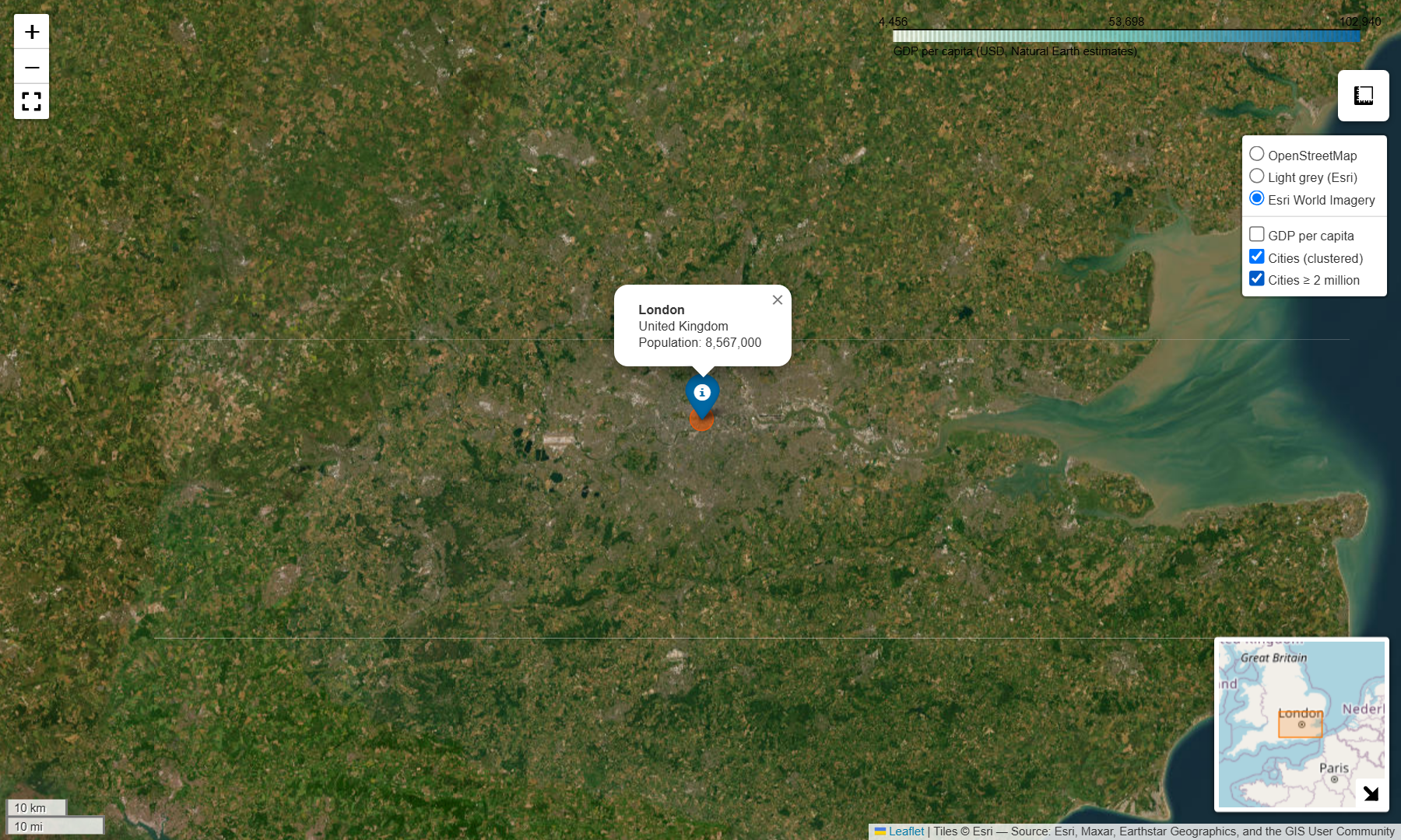
A FeatureGroup created with show=False appears unticked in the layer control. Here it holds circle markers scaled by population for cities over 2 million. Plugins add common web-map tools in one line each:
big = eu_places[eu_places["population"] >= 2_000_000]fg = folium.FeatureGroup(name="Cities ≥ 2 million", show=False).add_to(m)for _, r in big.iterrows():    folium.CircleMarker([r.geometry.y, r.geometry.x], radius=4 + r["population"] / 1.5e6,                        color="#e8590c", fill=True, fill_opacity=0.6, weight=1,                        tooltip=f"{r['city']}: {r['population']:,}").add_to(fg)
plugins.Fullscreen().add_to(m)plugins.MiniMap(toggle_display=True).add_to(m)plugins.MeasureControl(primary_length_unit="kilometers").add_to(m)folium.LayerControl(collapsed=False).add_to(m) # add this last so it sees every layerm.save("output/europe_folium.html")europe_folium.html 737 KBexplore_density.html 431 KB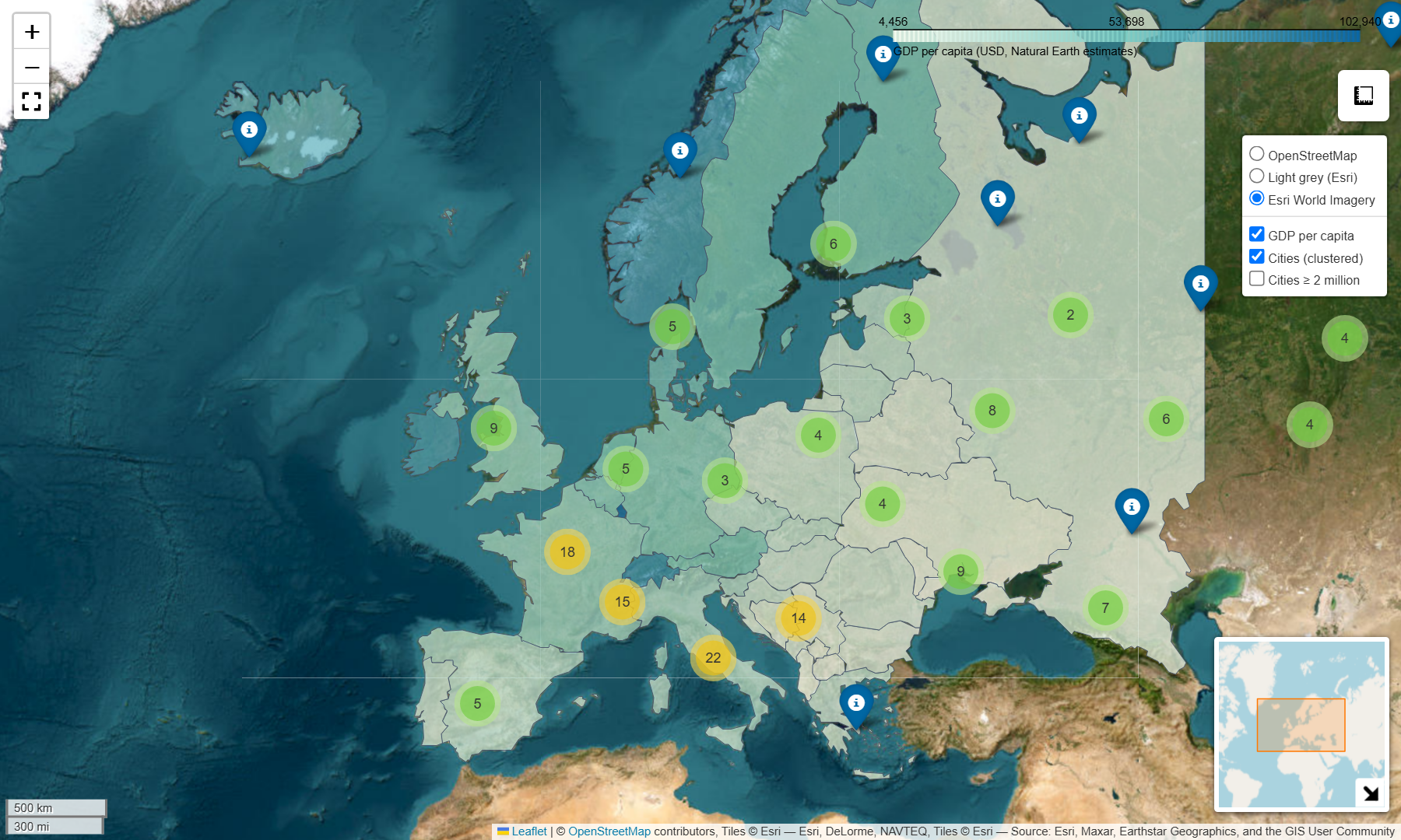
Try the live map
This is the exact europe_folium.html written by the script. Pan, zoom, switch layers and click the clusters:
Embedding and sharing tips
- Embed the HTML with an
<iframe>, as on this page, or usem._repr_html_()/m.get_root().render()if you need the markup as a string. - Big data? Folium embeds everything in the page, and a few thousand polygons is the practical limit. Beyond that, simplify harder, aggregate, or switch to vector tiles (PMTiles),
lonboardor a tile server. - Offline use: the HTML loads Leaflet and its plugins from CDNs and fetches tiles live, so it needs an internet connection to display.
- Attribution is shown automatically for built-in tile sets. Always pass
attr=for custom tile URLs.
Next steps
- Map the results of the OSMnx accessibility tutorial with
edges.explore(column="walk_min"). - Add a time slider with
plugins.TimestampedGeoJsonto animate the Lake Mead shoreline. - Prefer a static figure for print? See GeoPandas choropleths.
Data and licences
- Natural Earth 1:50m Admin 0 countries and populated places: public domain, naturalearthdata.com. Population and GDP are Natural Earth’s estimates.
- Basemaps: © OpenStreetMap contributors (ODbL); Esri World Light Gray Canvas (Esri, DeLorme, NAVTEQ); Esri World Imagery (Esri, Maxar, Earthstar Geographics and the GIS User Community).
- Code:
folium_maps.py, tested with Python 3.8.10, folium 0.18.0, geopandas 0.13.2 and mapclassify 2.6.0.
Key terms
- Folium
- A Python library that writes Leaflet.js web maps as HTML.
- Leaflet
- A lightweight open-source JavaScript library for interactive web maps.
- Basemap (tile layer)
- Background map imagery served as small XYZ tiles, such as OpenStreetMap or Esri World Imagery.
- Marker clustering
- Grouping nearby markers into numbered bubbles that split apart as you zoom in.
Data for this tutorial
- Natural Earth · Public-domain countries and populated places
- OpenStreetMap · ODbL 1.0
Licences and formats for each source are listed in the GIS data sources catalogue.