Street network analysis with OSMnx: routes, isochrones and walking accessibility
Download Sheffield's walkable street network from OpenStreetMap with OSMnx, find the shortest walk across the city, draw 5–20 minute isochrones and map how far every street is from the nearest supermarket.
- Level
- Intermediate
- Tested with
- Python 3.8
- Source code
- Download scripts
Key takeaways
- OSMnx downloads OpenStreetMap streets as a NetworkX graph; project it so edge lengths are in metres.
- The 20-minute walking isochrone from Sheffield station covers 4.44 km², a little over half the 8 km² circle a straight-line radius would suggest.
- One multi-source Dijkstra search gives every node its walking time to the nearest supermarket: two-thirds of the network is within 10 minutes and 8% is over 20 minutes away.
- Sheffield's street orientation entropy is 3.572, close to the 3.584 maximum: its streets follow valleys rather than a grid.
Before you start
- Basic GeoPandas (see the GeoPandas getting-started tutorial)
- Python 3.8+ with osmnx 1.9, networkx, geopandas, scipy and contextily
- An internet connection for the Overpass API (results are cached on disk after the first run)
Straight-line distance is the easiest measure in GIS, and often the wrong one. A shop 400 m away across a railway line or river might be a 15-minute walk. Real accessibility analysis needs a network. OSMnx by Geoff Boeing downloads OpenStreetMap streets as a routable NetworkX graph in one line, and converts it to and from GeoPandas whenever you need geometry.
In this tutorial we analyse central Sheffield and:
- download and project the walking network;
- compute the shortest walk from the railway station to the University;
- build walking isochrones, the areas reachable in 5, 10, 15 and 20 minutes;
- map walking time to the nearest supermarket for every street, using a multi-source Dijkstra search;
- plot a street orientation rose.
Every figure and number here was produced by sheffield_networks.py in October 2026. OpenStreetMap is continuously edited, so your counts will differ slightly.
Step 1: download the walking network
import osmnx as ox
ox.settings.use_cache = True                  # cache Overpass responses on diskCENTRE = (53.3801, -1.4703)                   # Peace Gardens, Sheffield (lat, lon)WALK_M_PER_MIN = 4.8 * 1000 / 60              # 4.8 km/h
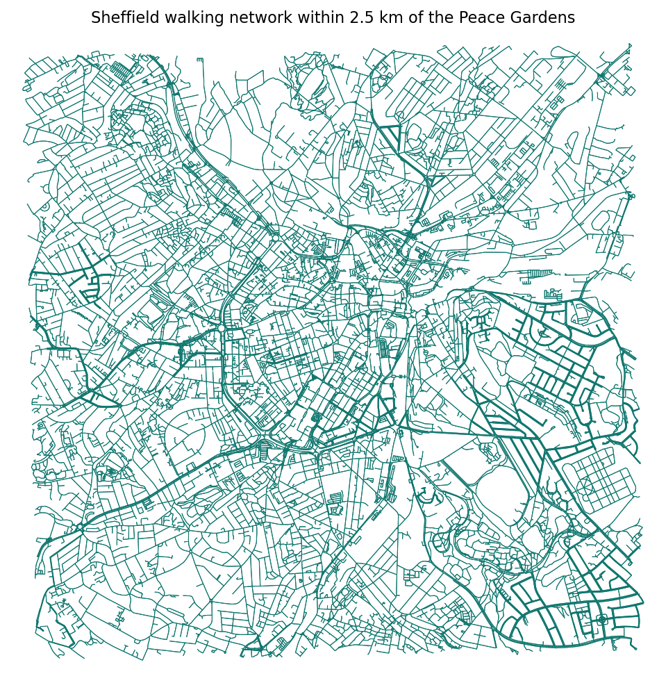
G = ox.graph_from_point(CENTRE, dist=2500, network_type="walk")Gp = ox.project_graph(G) # to local UTM so lengths/areas are in metresprint(Gp)print("crs:", Gp.graph["crs"])stats = ox.basic_stats(Gp)MultiDiGraph with 15103 nodes and 41542 edgescrs: EPSG:32630n 15,103m 41,542k_avg 5.50edge_length_total 1,601,151.72street_length_avg 38.54streets_per_node_avg 2.77intersection_count 12,128circuity_avg 1.06A few things to note:
network_type="walk"keeps footpaths, alleys and pedestrianised streets, and ignores one-way restrictions. The other options include"drive","bike"and"all".- The graph is a MultiDiGraph: each walkable street appears as two directed edges, which is why there are 41,542 edges and 1,601 km of total edge length. That is roughly 800 km of actual street.
project_graphchooses the local UTM zone (30N, EPSG:32630), so everylengthattribute is in metres.circuity_avgof 1.06 means streets are on average 6 % longer than the straight line between their ends.
Edges and nodes convert to GeoDataFrames with ox.graph_to_gdfs, so everything you know about GeoPandas applies:
nodes, edges = ox.graph_to_gdfs(Gp)print(edges[["osmid", "name", "highway", "length"]].head().to_string()) osmid name highway lengthu v key21026833 1056869084 0 91009446 NaN service 142.052 1234138844 0 [965944369, 965944375] Penistone Road trunk 56.910 69450069 0 965944370 Penistone Road trunk 84.3271056869084 1301711154 0 9264004 Capel Street unclassified 15.951 69450069 0 9264004 Capel Street unclassified 78.820The index is the (u, v, key) triple that identifies an edge in the graph. Simplified edges that merge several OSM ways keep a list of osmids.
Step 2: the shortest walk
To route between two places, we snap each point to its nearest graph node and then run Dijkstra’s algorithm, weighted by length:
pts = gpd.GeoSeries([Point(STATION[1], STATION[0]), Point(UNIVERSITY[1], UNIVERSITY[0])], crs="EPSG:4326").to_crs(Gp.graph["crs"])orig, dest = ox.distance.nearest_nodes(Gp, pts.x.tolist(), pts.y.tolist())route = ox.shortest_path(Gp, orig, dest, weight="length")route_gdf = ox.routing.route_to_gdf(Gp, route, weight="length")route_len = route_gdf["length"].sum()print(f"length: {route_len:,.0f} m | walking time: {route_len / WALK_M_PER_MIN:.1f} min")print("streets:", " → ".join(pd.unique(route_gdf["name"].dropna().astype(str))))nodes in route: 85length: 2,267 m | walking time: 28.3 minstreets: Sheaf Street → Shoreham Street → Grinders Hill → Brown Street → Furnival Street → Furnival Square → Furnival Gate → Wellington Street → Eldon Street → Devonshire Street → Fitzwilliam Street → Glossop Road → Hounsfield Road → Hounsfield Lane → Leavy Greave → University Concourse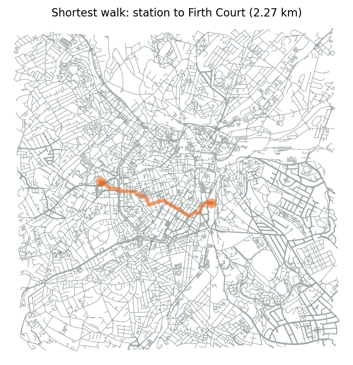
Step 3: walking isochrones
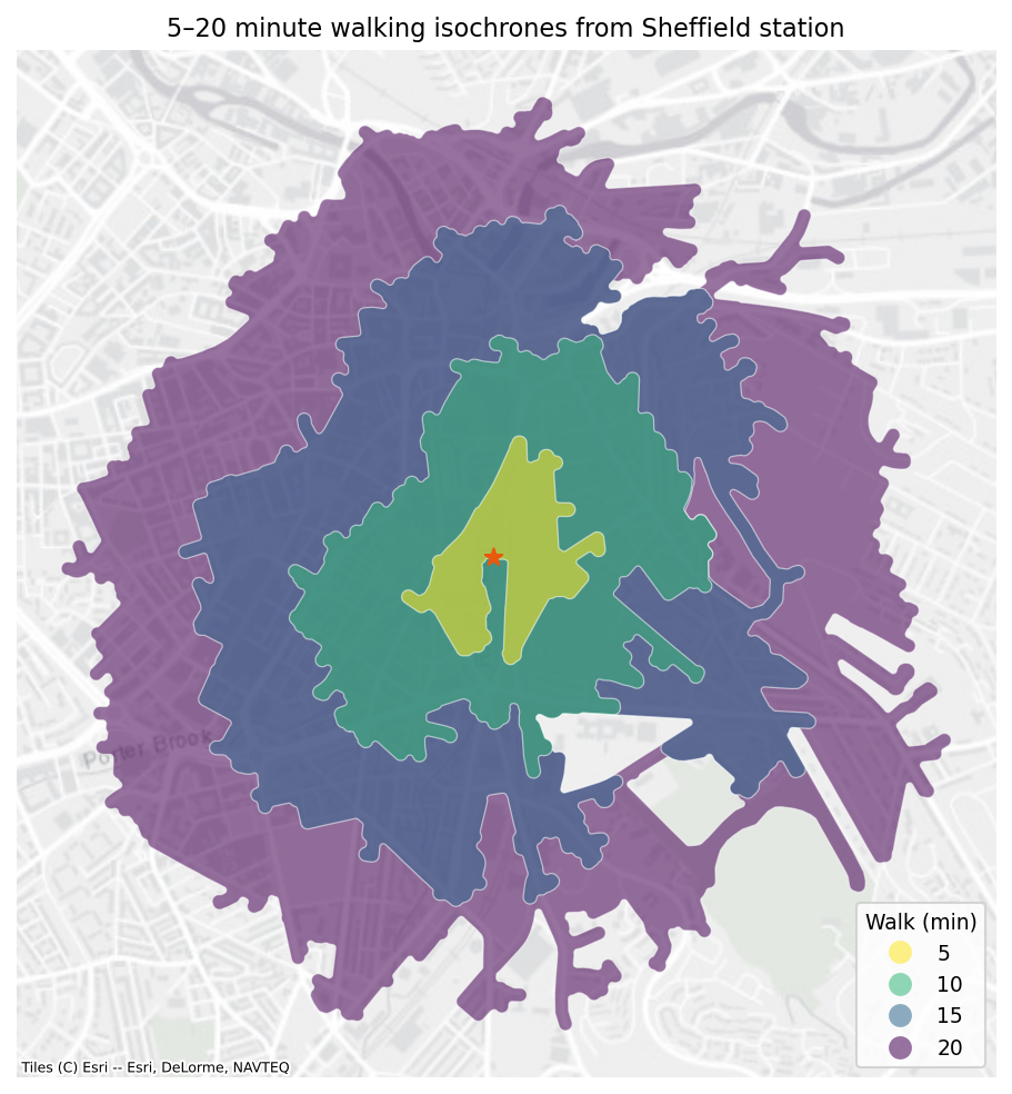
An isochrone is the area reachable within a given time. nx.ego_graph with distance="length" returns the subgraph within a network distance of a node. We buffer its edges and merge them into a polygon:
def fill_small_holes(geom, max_area=40_000):    """Remove interior rings (city blocks) smaller than max_area m²."""    polys = geom.geoms if isinstance(geom, MultiPolygon) else [geom]    out = [Polygon(p.exterior, [r for r in p.interiors if Polygon(r).area > max_area]) for p in polys]    return MultiPolygon(out) if len(out) > 1 else out[0]
isos = []for t in [20, 15, 10, 5]: sub = nx.ego_graph(Gp, orig, radius=t * WALK_M_PER_MIN, distance="length") sub_edges = ox.graph_to_gdfs(sub, nodes=False) isos.append({"minutes": t, "geometry": fill_small_holes(sub_edges.buffer(30).unary_union.buffer(-10))})iso = gpd.GeoDataFrame(isos, crs=Gp.graph["crs"])iso["area_km2"] = (iso.area / 1e6).round(2) minutes area_km2 5 0.17 10 0.96 15 2.32 20 4.44If walking were unconstrained, a 20-minute walk at 4.8 km/h would cover a circle of radius 1.6 km, or about 8 km². The network-based isochrone covers 4.44 km², a little over half of that. Railway lines, the inner ring road and the River Don all force detours. Buffering by 30 m and then shrinking by 10 m smooths the shape, while fill_small_holes removes the slivers inside city blocks but keeps genuinely unreachable areas, such as rail yards, as holes.
Step 4: how far is every street from a supermarket?
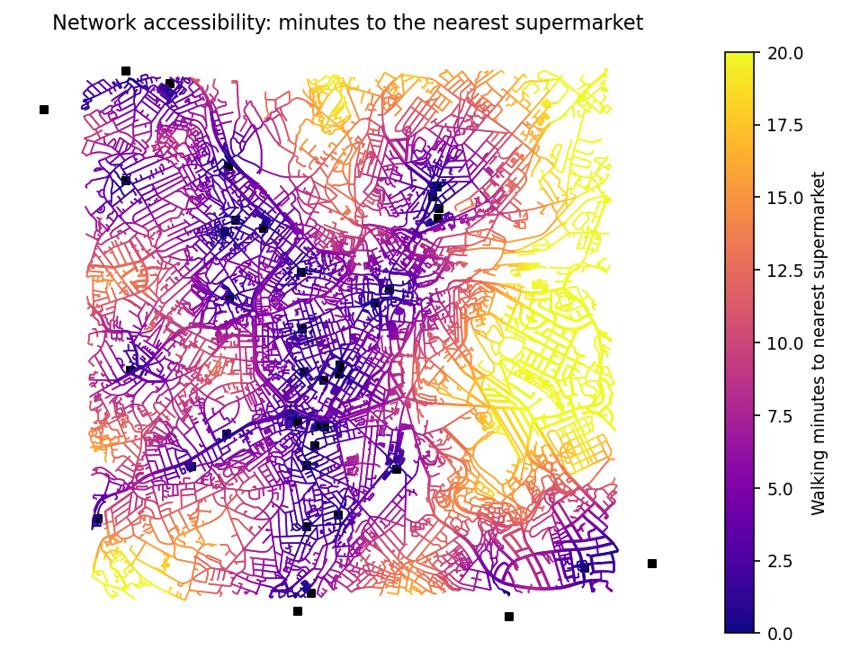
For accessibility analysis, we want the distance from every node to its nearest facility. Running Dijkstra once per supermarket would be slow. nx.multi_source_dijkstra_path_length does the job in a single pass, as if a virtual node were connected to all the shops:
shops = ox.features_from_point(CENTRE, tags={"shop": "supermarket"}, dist=3000)shops = shops.to_crs(Gp.graph["crs"])shops["geometry"] = shops.geometry.representative_point()  # polygons → pointsprint(len(shops), "supermarkets;", shops["name"].value_counts().head(6).to_dict())
shop_nodes = set(ox.distance.nearest_nodes(Gp, shops.geometry.x.tolist(), shops.geometry.y.tolist()))dist = nx.multi_source_dijkstra_path_length(Gp, shop_nodes, weight="length")nodes["walk_min"] = nodes.index.map(dist).astype(float) / WALK_M_PER_MIN38 supermarkets; {'Lidl': 3, 'Asda': 3, 'Heron Foods': 3, 'Morrisons': 2, 'Aldi': 2, 'Budgens': 1}ox.features_from_point returns any OSM features matching the tags, as either points or building polygons. representative_point() gives a point guaranteed to lie inside each polygon. Binning the result shows how much of the network falls within each walking band:
walk_min0–5 32.05–10 35.510–15 17.415–20 7.020+ 8.2Two-thirds of the network is within a 10-minute walk of a supermarket, but 8 % is more than 20 minutes away.
Step 5: street orientation
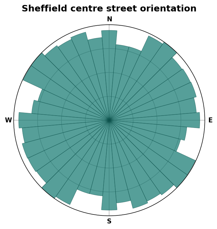
Finally, a polar histogram of street bearings, a favourite of urban morphologists:
Gu = ox.bearing.add_edge_bearings(ox.convert.to_undirected(G))fig, ax = ox.plot_orientation(Gu, title="Sheffield centre street orientation", area=True)print(round(ox.bearing.orientation_entropy(Gu), 3))3.572Orientation entropy, measured over 36 bins, ranges from about 1.39 for a perfect grid to ln(36) ≈ 3.584 for completely uniform bearings. Sheffield’s 3.572 is almost the maximum: its streets follow valleys and contours rather than a plan. A grid city such as Chicago scores far lower.
Summary
| Task | OSMnx / NetworkX |
|---|---|
| Download a network | ox.graph_from_point, graph_from_place, graph_from_polygon |
| Project to metres | ox.project_graph |
| To/from GeoPandas | ox.graph_to_gdfs, ox.graph_from_gdfs |
| Nearest node | ox.distance.nearest_nodes |
| Shortest path | ox.shortest_path, ox.routing.route_to_gdf |
| Reachable subgraph | nx.ego_graph(..., distance="length") |
| Distance to nearest facility | nx.multi_source_dijkstra_path_length |
| Save for QGIS | ox.save_graph_geopackage |
Next steps
- Add elevation to the edges with
ox.elevationand a DEM (see the terrain tutorial), then route by a hill-aware walking time using Tobler’s hiking function. - Turn the accessibility map into an interactive web map with Folium.
- Join the node walking times to census output areas, as in our bivariate census analysis.
Data and licences
- Street network and supermarkets: © OpenStreetMap contributors, available under the Open Database Licence (ODbL), downloaded via the Overpass API in October 2026.
- Basemap (isochrone figure): tiles © Esri — Esri, DeLorme, NAVTEQ (World Light Gray Canvas).
- Code:
sheffield_networks.py, tested with Python 3.8.10, osmnx 1.9.4 and networkx 3.1.
Key terms
- Isochrone
- The area reachable from a point within a given travel time over a network.
- Dijkstra search
- A shortest-path algorithm; the multi-source version finds the distance from every node to its nearest of several start points in one pass.
- MultiDiGraph
- A directed graph that allows several edges between the same two nodes; OSMnx stores each walkable street as two directed edges.
- Orientation entropy
- A measure of how evenly street bearings are spread across compass directions: low for a grid, high for organic street patterns.
Data for this tutorial
- OpenStreetMap · ODbL 1.0
- Geofabrik OpenStreetMap extracts · ODbL 1.0, by country and region
- GIS data sources for the United Kingdom
Licences and formats for each source are listed in the GIS data sources catalogue.