From DEM to 3D-printable STL with Python and NumPy

Our earlier post on creating a 3D-printed DEM in QGIS used QGIS plugins to turn terrain into something you can hold. This tutorial does the same job in about 100 lines of Python. The script is repeatable, so changing the area, scale or exaggeration is a one-line edit. It is also transparent: you’ll see exactly how a height grid becomes a closed triangle mesh, and you’ll verify that the mesh is watertight before you waste a spool of filament.

We’ll model the Edale valley in the Peak District. Kinder Scout’s plateau sits to the north and the Great Ridge (Mam Tor to Lose Hill) to the south, so there is plenty of relief in a 12 × 9 km box.

The steps are:

1. stream and reproject a Copernicus GLO-30 DEM;
2. convert metres to printable millimetres;
3. triangulate a closed solid (surface, base and walls) with vectorised NumPy;
4. check the mesh is watertight and consistently oriented;
5. write and re-read a binary STL.

Only NumPy and rioxarray are needed: no mesh library. The full script is dem_to_stl.py.

Step 1: get the DEM in a metric CRS

The Copernicus DEM is published as one cloud-optimised GeoTIFF per 1° tile on AWS. rioxarray reads only the bytes it needs. We clip a generous lon/lat window, reproject to British National Grid so that every cell is a true 30 × 30 m square, and then clip the exact study area:

DEM_URL = ("https://copernicus-dem-30m.s3.amazonaws.com/"
           "Copernicus_DSM_COG_10_N53_00_W002_00_DEM/Copernicus_DSM_COG_10_N53_00_W002_00_DEM.tif")
AOI_BNG = (406_000, 380_000, 418_000, 389_000)   # 12 x 9 km: Kinder plateau, Edale, Mam Tor

dem = rioxarray.open_rasterio(DEM_URL, masked=True).squeeze("band", drop=True)
dem = dem.rio.clip_box(-1.95, 53.30, -1.70, 53.45).load()            # generous lon/lat window
dem = dem.rio.reproject("EPSG:27700", resolution=30, resampling=Resampling.bilinear)
dem = dem.rio.clip_box(*AOI_BNG)
z = dem.values.astype("float64")

=== DEM ===
shape (rows, cols): (301, 401) | resolution: (30.0, -30.0)
NaNs: 0
elevation range: 158.0 - 634.5 m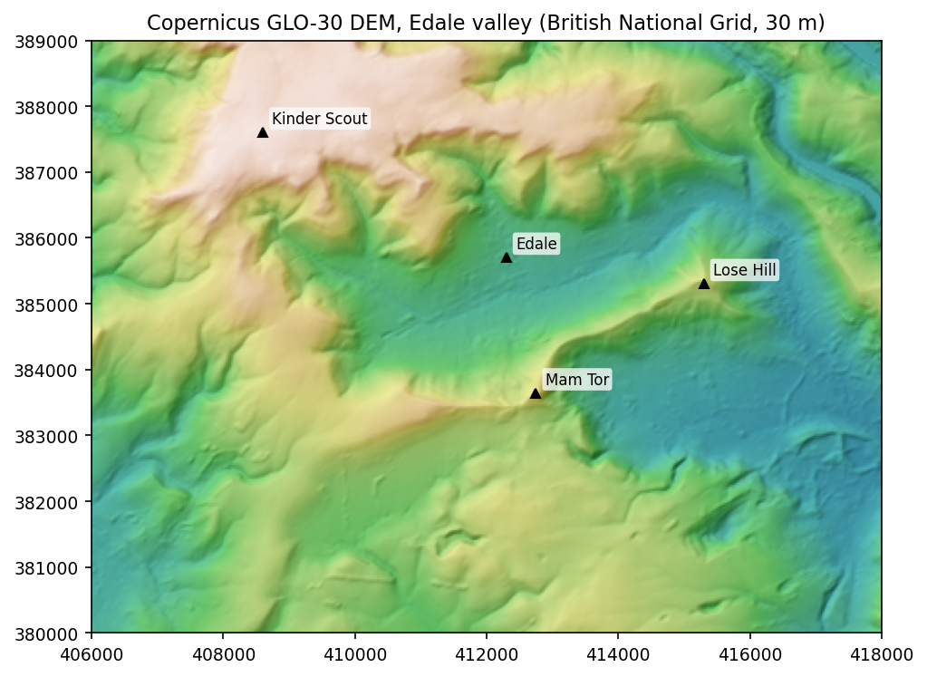

Reprojecting first matters. In geographic coordinates a 1-arc-second cell is about 31 m north–south but only about 18 m east–west at 53°N. A mesh built on those cells would be squashed. If you prefer, the raster tutorial covers this data source and reprojection in more depth.

Step 2: from metres to millimetres

A printer works in millimetres, so we choose the printed size of the longest side and derive everything else from it. A vertical exaggeration of 2x makes moderate relief readable, and a 4 mm plinth gives the model a solid base:

MODEL_WIDTH_MM = 150.0
Z_EXAGGERATION = 2.0
BASE_MM = 4.0

rows, cols = z.shape
cell_m = abs(dem.rio.resolution()[0])
width_m, height_m = (cols - 1) * cell_m, (rows - 1) * cell_m
scale = MODEL_WIDTH_MM / max(width_m, height_m)        # mm per metre

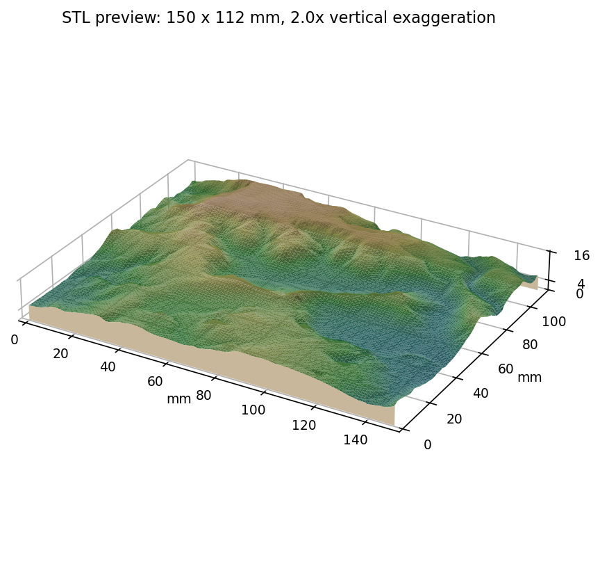
x = np.arange(cols) * cell_m * scale
y = (rows - 1 - np.arange(rows)) * cell_m * scale    # row 0 is north -> largest y
X, Y = np.meshgrid(x, y)
Z = BASE_MM + (z - np.nanmin(z)) * scale * Z_EXAGGERATION

=== model scale ===
ground extent: 12.00 x 9.00 km
horizontal scale: 1:80,000
cell size on the print: 0.375 mm
model size: 150.0 x 112.5 x 15.9 mm (W x D x H)

A 0.375 mm cell is close to a typical 0.4 mm nozzle width, so the 30 m DEM is a good match for this print size. Finer data would add triangles without adding printable detail.

Step 3: triangulate a closed solid

An STL is just a list of triangles. To be printable, the triangles must enclose a volume with no holes: the mesh must be watertight. We build three parts.

The surface. Each grid cell becomes two triangles. Rather than looping over 120,000 cells, we compute the four corner indices of every cell as arrays:

def grid_triangles(r: int, c: int) -> np.ndarray:
    """Vertex indices for two counter-clockwise triangles per grid cell (viewed from above)."""
    idx = np.arange(r * c).reshape(r, c)
    a, b = idx[:-1, :-1].ravel(), idx[:-1, 1:].ravel()   # top-left, top-right
    d, e = idx[1:, :-1].ravel(), idx[1:, 1:].ravel()     # bottom-left, bottom-right
    # y decreases with row, so (a, d, b) and (b, d, e) are anticlockwise from above
    return np.concatenate([np.column_stack([a, d, b]), np.column_stack([b, d, e])])

The base. We copy every vertex at z = 0 and reuse the same triangles with the winding reversed, so their normals point down:

top_v = np.column_stack([X.ravel(), Y.ravel(), Z.ravel()])
bot_v = top_v.copy()
bot_v[:, 2] = 0.0
verts = np.vstack([top_v, bot_v])
n = rows * cols
tri_top = grid_triangles(rows, cols)
tri_bottom = tri_top[:, ::-1] + n                         # reversed winding -> faces down

The walls. We walk the outer ring of grid vertices clockwise (seen from above) and join each edge to the matching base edge with two triangles:

idx = np.arange(n).reshape(rows, cols)
ring = np.concatenate([idx[0, :], idx[1:, -1], idx[-1, -2::-1], idx[-2:0:-1, 0]])
p, q = ring, np.roll(ring, -1)
walls = np.concatenate([np.column_stack([p, q, p + n]), np.column_stack([q, q + n, p + n])])
triangles = np.vstack([tri_top, tri_bottom, walls])

=== mesh ===
vertices: 241,402  triangles: 482,800 (surface 240,000, base 240,000, walls 2,800)

The counts check out: 400 × 300 cells × 2 = 240,000 surface triangles, and the ring has 2 × (401 + 301) − 4 = 1,400 edges, each producing 2 wall triangles.

Step 4: prove it’s printable

Slicers will often “repair” a broken mesh silently, so it is better to check it yourself. A closed, consistently oriented triangle mesh has two properties that are easy to test with np.unique:

• every undirected edge is shared by exactly two triangles (no holes or flaps);
• every directed edge appears exactly once, because a neighbouring triangle traverses the shared edge in the opposite direction (consistent winding).

edges = np.concatenate([triangles[:, [0, 1]], triangles[:, [1, 2]], triangles[:, [2, 0]]])
_, und_counts = np.unique(np.sort(edges, axis=1), axis=0, return_counts=True)
_, dir_counts = np.unique(edges, axis=0, return_counts=True)
print("watertight:", bool((und_counts == 2).all()), "| consistently oriented:", bool((dir_counts == 1).all()))

tri_xyz = verts[triangles]                                 # (n_tri, 3 vertices, xyz)
normals = np.cross(tri_xyz[:, 1] - tri_xyz[:, 0], tri_xyz[:, 2] - tri_xyz[:, 0])
volume_mm3 = np.einsum("ij,ij->i", tri_xyz[:, 0], np.cross(tri_xyz[:, 1], tri_xyz[:, 2])).sum() / 6

The volume uses the divergence theorem: sum the signed volumes of the tetrahedra formed by each triangle and the origin. A positive total confirms the normals face outwards. If they faced inwards, the total would be negative.

watertight: True | consistently oriented: True
enclosed volume: 156.2 cm³ (positive = outward-facing normals)

Step 5: write a binary STL with NumPy

The binary STL format is simple:

• an 80-byte header;
• a uint32 triangle count;
• 50 bytes per triangle: a normal (3 × float32), three vertices (9 × float32) and a 2-byte attribute.

A NumPy structured dtype describes that layout exactly, so the whole file is written in one call:

lengths = np.linalg.norm(normals, axis=1, keepdims=True)
unit = np.divide(normals, lengths, out=np.zeros_like(normals), where=lengths > 0)
record = np.dtype([("normal", "<f4", 3), ("v", "<f4", (3, 3)), ("attr", "<u2")])
data = np.zeros(len(triangles), dtype=record)
data["normal"], data["v"] = unit, tri_xyz
with open(stl_path, "wb") as f:
    f.write(b"TechnicalGIS Edale DEM - Copernicus GLO-30".ljust(80, b" "))
    f.write(np.uint32(len(data)).tobytes())
    f.write(data.tobytes())

Then we read the file back with the same dtype to prove it is valid:

=== STL ===
wrote edale_kinder_mam_tor.stl: 24.1 MB, 482,800 facets
read back: 482800 facets | bounding box (mm): [0. 0. 0.] -> [150.  112.5  15.9]

84 + 482,800 × 50 bytes = 24.1 MB, exactly as expected. The bounding box is the model size we designed in step 2.

Printing tips

• Orientation: print flat on the plinth. The surface has no overhangs, so no supports are needed.
• Layer height: 0.1–0.15 mm layers capture the subtle valley floor. At 0.3 mm the gentle Hope Valley floor, under 1 mm above the plinth, becomes a few visible steps.
• Infill: 10–15 % is plenty, since the plinth and walls do the structural work.
• File size: at 24 MB the STL is fine for any slicer. To share it, export to 3MF or decimate it in MeshLab or Blender.
• Bigger areas: keep the cell size on the print around 0.3–0.5 mm by resampling the DEM, e.g. dem.rio.reproject(..., resolution=60) to cover twice the ground extent at the same print size.

Next steps

• Add a second material layer: rasterise rivers or lakes and lower them by 0.5 mm, so you can pause and swap filament colour.
• Combine this with the OSMnx tutorial to emboss a walking route onto the terrain.
• Compare with the QGIS approach and see which workflow suits you.

Data and licences

• Copernicus DEM GLO-30: © DLR e.V. 2010–2014 and © Airbus Defence and Space GmbH 2014–2018, provided under COPERNICUS by the European Union and ESA; all rights reserved. Accessed from the AWS Open Data registry.
• Code: dem_to_stl.py, tested with Python 3.8.10, numpy 1.23.4, rasterio 1.3.11 and rioxarray 0.13.4.