Getting started with GeoPandas: projections, spatial joins and choropleth maps
Load Natural Earth vector data with GeoPandas, reproject to an equal-area CRS, calculate population density, join cities to countries, dissolve to continents and draw publication-ready choropleths.
- Level
- Beginner
- Tested with
- Python 3.8
- Source code
- Download scripts
Key takeaways
- A GeoDataFrame is a pandas DataFrame with a geometry column and a CRS, so vector GIS operations sit alongside ordinary pandas code.
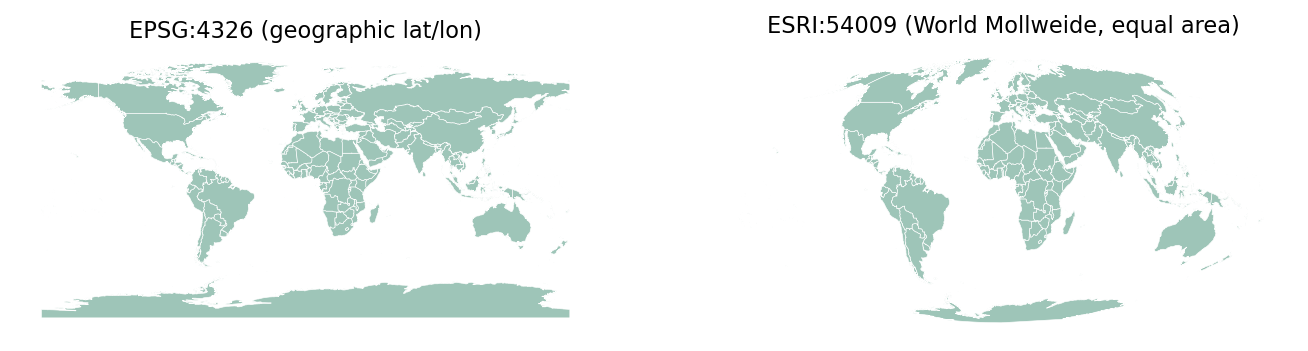
- Reproject before you measure: areas in EPSG:4326 are in square degrees, so use an equal-area projection such as World Mollweide for global areas.
- sjoin() attaches attributes by location. Count the unmatched rows afterwards: 7% of Natural Earth cities, mostly coastal, missed a country until sjoin_nearest() was used.
- dissolve() is a spatial groupby, and plot(column=..., scheme=...) draws a classified choropleth in one call.
Before you start
- Python 3.8 or newer with pip and a virtual environment
- Basic pandas: selecting columns, groupby
- Around 10 MB of disk space for the Natural Earth downloads
If you have used QGIS or ArcGIS Pro, you already know the core operations of vector GIS: reprojecting, calculating areas, joining layers by location and dissolving boundaries. GeoPandas gives you the same operations in Python. Because a GeoDataFrame is a pandas DataFrame with a geometry column, your analysis becomes a script you can re-run, review and schedule.
In this tutorial we will use free Natural Earth data to:
- read country polygons and city points straight from a zip file;
- reproject them to an equal-area coordinate reference system (CRS) so areas are correct;
- map population density as a choropleth;
- attach a country to every city with a spatial join, and fix the cities that miss;
- dissolve countries into continents and save everything to a GeoPackage.
Every number and figure below came from running geopandas_basics.py.
Set up the environment
Create a fresh virtual environment and install the pinned versions we tested with:
python -m venv .venv.venv\Scripts\activate # macOS/Linux: source .venv/bin/activatepip install geopandas==0.13.2 shapely==2.0.7 pyogrio==0.9.0 pandas==2.0.3 matplotlib==3.7.5 mapclassify==2.6.0mapclassify gives GeoDataFrame.plot() its classification schemes (quantiles, natural breaks and so on). pyogrio is the fast GDAL-based reader that GeoPandas 1.x now uses by default.
Step 1: read the data
GeoPandas can read a zipped shapefile directly, so there is no need to unzip it first. The script downloads two Natural Earth 1:50m layers once and caches them in ./data:
import geopandas as gpd
countries = gpd.read_file(fetch("ne_50m_admin_0_countries.zip"))places = gpd.read_file(fetch("ne_50m_populated_places.zip"))
print(type(countries))print(countries.shape)print(countries.crs)print(countries.geom_type.value_counts())<class 'geopandas.geodataframe.GeoDataFrame'>(242, 169)EPSG:4326Polygon 123MultiPolygon 119Name: count, dtype: int64There are 242 countries and 169 attribute columns. The CRS is EPSG:4326, plain longitude and latitude in degrees. Almost half the features are MultiPolygons: any country with islands or exclaves is stored as several parts.
Most of those 169 columns are labels in other languages, so keep only what we need and give the columns friendlier names:
countries = countries[["NAME", "ISO_A3_EH", "CONTINENT", "POP_EST", "GDP_MD", "geometry"]]countries = countries.rename(columns={"NAME": "name", "ISO_A3_EH": "iso3", "CONTINENT": "continent", "POP_EST": "pop_est", "GDP_MD": "gdp_musd"})print(countries.head()) name iso3 continent pop_est gdp_musd geometry0 Zimbabwe ZWE Africa 14645468.0 21440 POLYGON ((31.28789 -22.40205, 31.19727 -22.344...1 Zambia ZMB Africa 17861030.0 23309 POLYGON ((30.39609 -15.64307, 30.25068 -15.643...2 Yemen YEM Asia 29161922.0 22581 MULTIPOLYGON (((53.08564 16.64839, 52.58145 16...3 Vietnam VNM Asia 96462106.0 261921 MULTIPOLYGON (((104.06396 10.39082, 104.08301 ...4 Venezuela VEN South America 28515829.0 482359 MULTIPOLYGON (((-60.82119 9.13838, -60.94141 9...Step 2: reproject before you measure
countries.area in EPSG:4326 would return square degrees, which mean nothing, because a degree of longitude shrinks towards the poles. To measure areas, reproject to an equal-area projection first. World Mollweide (ESRI:54009) works well for global data:
countries_ea = countries.to_crs("ESRI:54009")  # World Mollweide (equal area)countries_ea["area_km2"] = countries_ea.area / 1e6countries_ea["density"] = countries_ea["pop_est"] / countries_ea["area_km2"]
print(countries_ea.nlargest(5, "area_km2")[["name", "area_km2", "pop_est", "density"]].round(1).to_string(index=False)) name area_km2 pop_est density Russia 16913027.1 144373535.0 8.5 Antarctica 12126825.6 4490.0 0.0 Canada 9894148.9 37589262.0 3.8United States of America 9460566.8 328239523.0 34.7 China 9392194.5 1397715000.0 148.8These areas are within a few percent of the official figures; Russia’s official area is about 17.1 million km². The 1:50m coastlines are generalised, so small islands and intricate coasts lose a little area.
Step 3: a choropleth in one call
With mapclassify installed, plot() can classify a column and draw a legend in one call. Quantile classes suit skewed data like population density, which runs from almost zero in Greenland to tens of thousands per km² in city-states:
world = countries_ea[countries_ea["continent"] != "Antarctica"]fig, ax = plt.subplots(figsize=(10, 5))world.plot(column="density", scheme="Quantiles", k=6, cmap="YlGnBu", legend=True, edgecolor="white", linewidth=0.25, ax=ax, legend_kwds={"title": "People per km²", "loc": "lower left", "fmt": "{:.0f}", "fontsize": 7})ax.set_title("Population density by country (quantile classes)")ax.set_axis_off()fig.savefig("output/02-density-choropleth.png")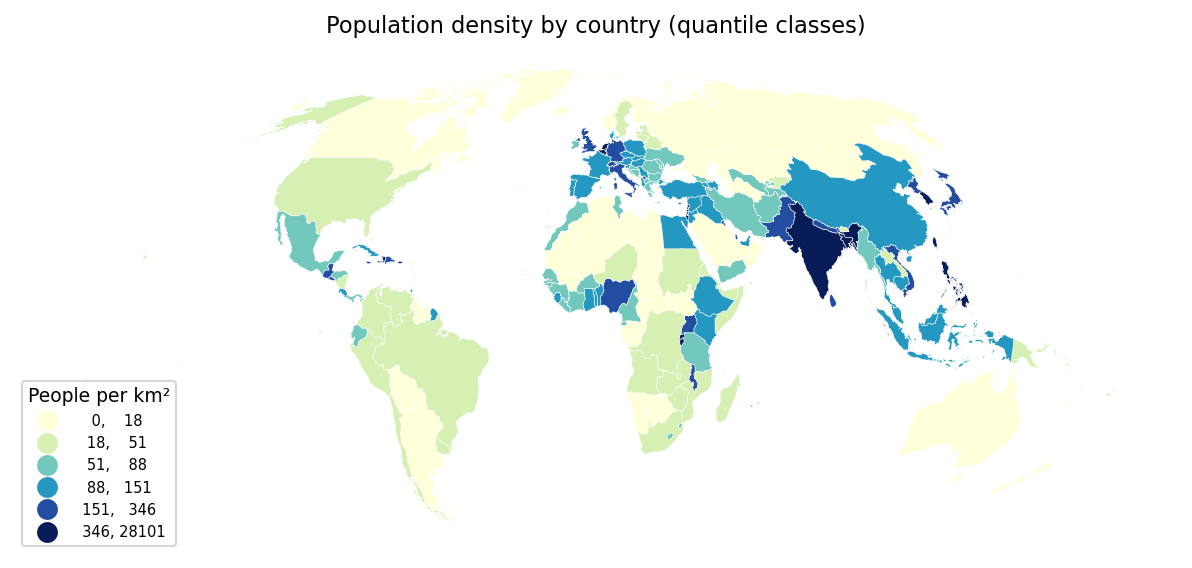
Step 4: spatial joins — which country is each city in?
The populated places layer has 1,251 points but no reliable country column. gpd.sjoin() adds one by testing every point against every polygon. GeoPandas uses a spatial index, so this takes milliseconds rather than the 300,000 brute-force tests it would otherwise need. Both layers must use the same CRS:
places = places[["NAME", "POP_MAX", "geometry"]].rename(columns={"NAME": "city", "POP_MAX": "city_pop"})places_ea = places.to_crs(countries_ea.crs)joined = gpd.sjoin(places_ea, countries_ea[["name", "continent", "geometry"]], how="inner", predicate="within")
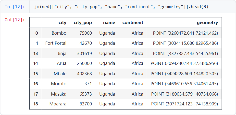
print(joined[["city", "city_pop", "name", "continent"]].head().to_string())print(len(places_ea) - len(joined), "of", len(places_ea), "places fall outside every country polygon") city city_pop name continent0 Bombo 75000 Uganda Africa1 Fort Portal 42670 Uganda Africa13 Jinja 301619 Uganda Africa14 Arua 250000 Uganda Africa15 Mbale 402368 Uganda Africa
94 of 1251 places fall outside every country polygonIn a notebook the joined GeoDataFrame renders as a table. Columns from the right-hand layer (name, continent) now sit next to each city, and the index is preserved, which is why it jumps from 1 to 13:
Fixing the points that miss
Seven percent of places matched nothing. Look at which ones and the pattern is clear: they are coastal cities. Natural Earth’s 1:50m coastline is simplified, so a city on the shore can sit a few hundred metres out to sea. sjoin_nearest() handles this. It assigns each leftover point to the closest polygon within a distance limit and reports how far away it was:
unmatched = places_ea[~places_ea.index.isin(joined.index)]nearest = gpd.sjoin_nearest(unmatched, countries_ea[["name", "continent", "geometry"]], max_distance=25_000, distance_col="dist_m")print(len(nearest), "recovered within 25 km")print(nearest.nlargest(5, "city_pop")[["city", "city_pop", "name", "dist_m"]].round(0).to_string())joined = pd.concat([joined, nearest.drop(columns="dist_m")])92 recovered within 25 km city city_pop name dist_m1226 New York 19040000 United States of America 1478.01228 Istanbul 10061000 Turkey 869.01233 Lagos 9466000 Nigeria 1576.01250 Hong Kong 7206000 Hong Kong 1327.01171 Salvador 3484000 Brazil 927.0New York, Istanbul, Lagos and Hong Kong, some of the largest cities on Earth, would have silently vanished from a simple within join, yet each lies less than 2 km from the generalised coastline. Always count your unmatched rows after a spatial join.
Now we can aggregate as in plain pandas, for example to count the cities with more than a million people in each country:
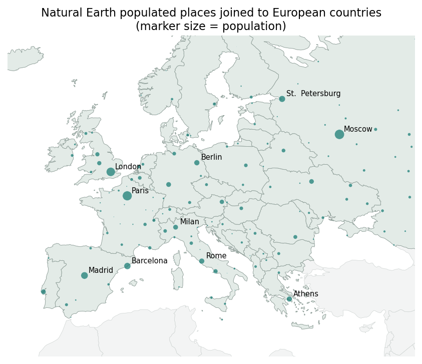
big = joined[joined["city_pop"] >= 1_000_000]per_country = big.groupby("name").agg(cities_1m=("city", "count"), city_pop=("city_pop", "sum"))print(per_country.sort_values("cities_1m", ascending=False).head(8)) cities_1m city_popnameChina 67 198833000India 42 140258000United States of America 40 132086838Brazil 18 71900406Russia 11 25533000Japan 8 61636000Nigeria 7 20462000Indonesia 7 20886000Use the .cx[] coordinate indexer to clip to a bounding box and map Europe’s cities, with marker size scaled by population:
Step 5: dissolve countries into continents
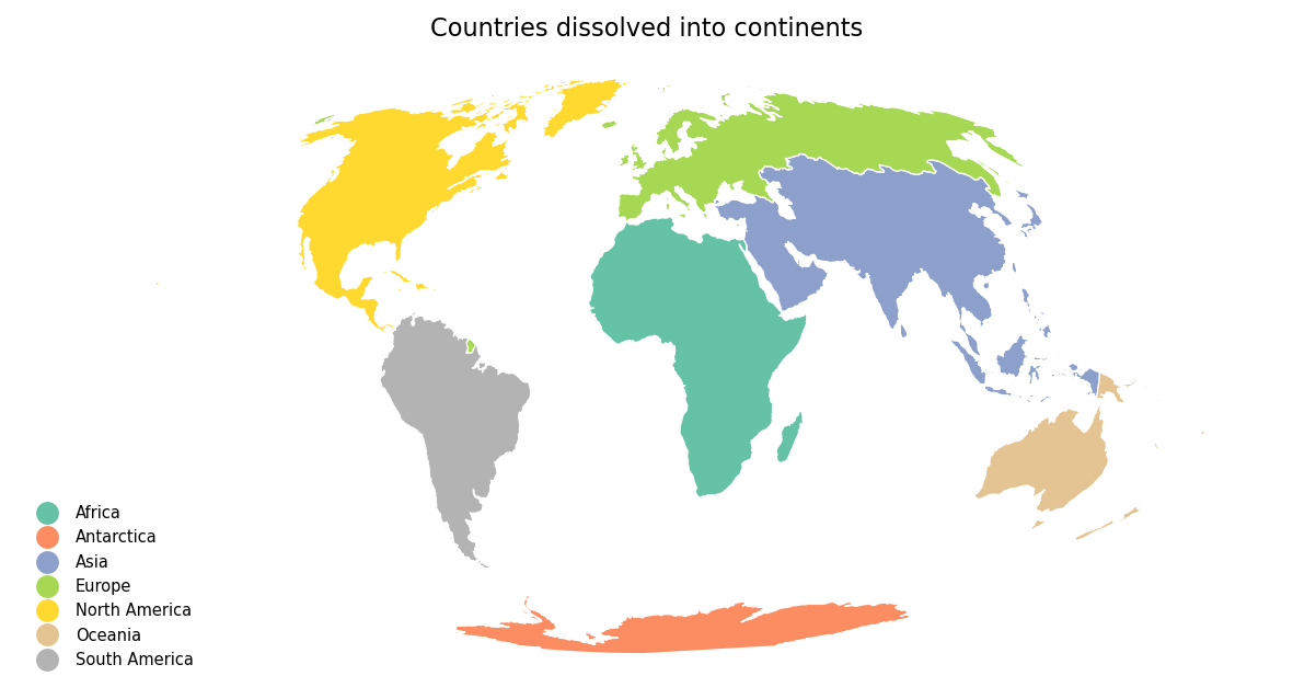
dissolve() is GeoPandas’ group by for geometry. It merges polygons that share a value and aggregates the other columns:
continents = countries_ea[countries_ea["continent"] != "Seven seas (open ocean)"].dissolve( by="continent", aggfunc={"pop_est": "sum", "gdp_musd": "sum", "area_km2": "sum"})continents["density"] = continents["pop_est"] / continents["area_km2"]print(continents.drop(columns="geometry").sort_values("pop_est", ascending=False)) pop_est gdp_musd area_km2 densitycontinentAsia 4,565,778,126.0 33555734 31,231,657.3 146.2Africa 1,307,986,092.3 2459078 30,053,513.8 43.5Europe 746,437,653.0 21642328 22,900,334.1 32.6North America 585,351,846.0 25115795 24,230,324.1 24.2South America 427,066,661.0 3852015 17,702,395.3 24.1Oceania 42,430,881.0 1663441 8,539,629.5 5.0Antarctica 4,490.0 898 12,126,825.6 0.0Europe’s 22.9 million km² is much larger than you might expect because Natural Earth assigns all of Russia, including Siberia, to Europe. Check how a dataset defines its groups before you quote aggregated figures.
Step 6: save the results
GeoPackage is a single-file, open-standard format that holds several layers, with none of the shapefile’s 10-character column-name limit:
gpkg = OUT / "natural_earth_analysis.gpkg"countries_ea.to_file(gpkg, layer="countries", driver="GPKG")continents.to_file(gpkg, layer="continents", driver="GPKG")joined.drop(columns="index_right").to_file(gpkg, layer="places_joined", driver="GPKG")natural_earth_analysis.gpkg 3.12 MBDrag the .gpkg into QGIS and you will see all three layers, already in Mollweide.
What you learned
- A
GeoDataFrameis a pandas DataFrame plus a geometry column and a CRS. - Reproject before measuring: use an equal-area CRS for areas and a local projected CRS for distances.
sjoin()joins by location; count the unmatched rows and usesjoin_nearest()for points that fall just outside polygons.dissolve()is a spatialgroupby.plot(column=..., scheme=...)gives you a classified choropleth in one line.
Next steps
- Speed up joins and overlays on millions of features in Fast vector geoprocessing with Shapely 2 and GeoParquet.
- Turn these GeoDataFrames into interactive maps in Interactive web maps with Folium.
- Find national boundary data for almost every country in our GIS data sources catalogue.
Data and licences
- Admin 0 countries and populated places, 1:50m: Natural Earth, public domain. Downloaded from
naciscdn.orgin October 2026; population estimates are those bundled with the dataset. - Code:
geopandas_basics.py, tested with Python 3.8.10, GeoPandas 0.13.2, Shapely 2.0.7 and pandas 2.0.3. Newer GeoPandas 1.x releases run it unchanged.
Key terms
- CRS
- A coordinate reference system defines how coordinates map to places on Earth, for example EPSG:4326 (longitude/latitude) or ESRI:54009 (World Mollweide).
- Equal-area projection
- A map projection that preserves the relative size of areas, so area calculations are meaningful.
- Spatial join
- A join that matches rows by the spatial relationship of their geometries (within, intersects, nearest) rather than by a shared key.
- Choropleth
- A map that shades areas according to a classified attribute value, such as population density.
Data for this tutorial
- Natural Earth · Public-domain countries and populated places
- Boundary data for every country
Licences and formats for each source are listed in the GIS data sources catalogue.