Monitoring reservoir water quality from space with Sentinel-2 and Python (Peak District case study)

Short answer: to monitor reservoir water quality with Sentinel-2 in Python, search the free Sentinel-2 L2A archive with STAC, mask cloud and shadow with the SCL band, keep only clear water pixels well inside the shoreline, and compute indices from the median water spectrum on each date. Use NDCI = (B5 − B4) / (B5 + B4) as a chlorophyll-a proxy, NDTI or red reflectance as a turbidity proxy, and a band ratio such as B3 / B2 for colour. Then compare each date with the reservoir’s normal for that month. These are relative indices: without local calibration and a water-specific atmospheric correction, they flag when and where to look, not how many µg/L of chlorophyll are present.

The Peak District reservoirs supply drinking water to Sheffield, Derby, Nottingham, Leicester and Manchester. Like most upland reservoirs in Britain, they are small, narrow, steep-sided and stained brown by peat. That makes them a hard, realistic test for satellite water-quality monitoring. In this tutorial we follow four of them from January 2019 to October 2026: Howden, Derwent and Ladybower in the Upper Derwent Valley (Severn Trent), and Torside in Longdendale (United Utilities), using every Sentinel-2 image of the area.

You will learn how to:

1. get reservoir outlines from OpenStreetMap with osmnx, and shrink them to avoid mixed shoreline pixels;
2. search and stream Sentinel-2 L2A from the Microsoft Planetary Computer, handling the processing-baseline offset;
3. build a cloud, shadow and water mask that works for dark, peaty water, and see why MNDWI does not;
4. compute NDCI, MCI, NDTI and a colour ratio, with quality control;
5. build a multi-year time series, a monthly climatology and a ranked list of anomalous dates;
6. map NDCI and turbidity for one date and export a tidy CSV per reservoir;
7. check the results against public Environment Agency samples.

All outputs below are real results from reservoir_water_quality.py, run on 15 October 2026 with Python 3.12, pystac-client 0.9.0, rasterio 1.5.2 and osmnx 2.1.1.

What can a satellite see in a reservoir?

A satellite sees only the light that leaves the water surface. Several things in the water change its colour:

• Chlorophyll-a in algae absorbs red light near 665 nm (Sentinel-2 band B4) and, as algae build up, causes a reflectance peak near 705 nm (B5). NDCI and MCI measure that peak.
• Suspended sediment scatters light and raises reflectance, most visibly in the red (B4). NDTI compares red with green.
• Coloured dissolved organic matter (CDOM), the brown stain from peat, absorbs blue light strongly and makes the water very dark. It is a real water-treatment issue in the Peak District, because colour must be removed before the water can be supplied.

Sentinel-2 has 10–20 m pixels, a red-edge band at 705 nm and a revisit of 2–5 days, which makes it the best free sensor for small lakes. Sentinel-3 OLCI has better water bands but 300 m pixels, wider than these reservoirs. Landsat 8 and 9 have no red-edge band, so they cannot compute NDCI.

Step 1: get the reservoir outlines from OpenStreetMap

OpenStreetMap maps reservoirs with the tag water=reservoir. osmnx downloads every matching polygon in a bounding box from the Overpass API. Public Overpass servers are often busy, so the script retries with backoff and a mirror, and caches the result in a GeoPackage:

RESERVOIRS = ["Howden", "Derwent", "Ladybower", "Torside"]   # north to south, then Longdendale
CRS = "EPSG:32630"            # UTM zone 30N, the native grid of Sentinel-2 tile 30UWE
INSET_M = 40                  # shrink each outline by 40 m (two 20 m pixels) to avoid mixed shoreline pixels

osm = ox.features_from_bbox((-1.95, 53.33, -1.62, 53.55), {"water": "reservoir"})
osm = osm[osm.geometry.type.isin(["Polygon", "MultiPolygon"]) & osm["name"].notna()]
osm = osm[osm["name"].isin([f"{r} Reservoir" for r in RESERVOIRS])].reset_index()

res = gpd.read_file(outlines).to_crs(CRS)
res["reservoir"] = res["name"].str.replace(" Reservoir", "")
res = res.dissolve("reservoir").loc[RESERVOIRS].reset_index()
res["core"] = res.buffer(-INSET_M)

The negative buffer is important. A 20 m pixel on the shoreline mixes water with grass, rock or trees, which are hundreds of times brighter in the near-infrared and red edge. Even one such pixel can dominate a water index. Shrinking each outline by 40 m keeps only pixels that are entirely water.

reservoir      id  area_ha  core_ha
   Howden  955357     62.4     33.6
  Derwent  955161     69.5     42.9
Ladybower 1959653    198.1    124.8
  Torside 8598540     62.6     42.0

The inset removes 33–46% of each reservoir’s area. That is the price of working with long, narrow lakes. We then rasterise the cores onto one 20 m grid that covers all four reservoirs:

817 x 738 pixels of 20 m (16.3 x 14.8 km), EPSG:32630
Howden       838 core water pixels
Derwent     1073 core water pixels
Ladybower   3129 core water pixels
Torside     1046 core water pixels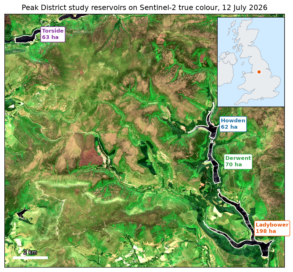

Step 2: search the Sentinel-2 archive with STAC

The Microsoft Planetary Computer holds the whole Sentinel-2 L2A archive as Cloud Optimised GeoTIFFs. All four reservoirs fall inside one tile, 30UWE, so we search for that tile only. A few dates appear twice, once from the original processing and once from ESA’s reprocessing, so we keep one scene per date and orbit:

STAC_URL = "https://planetarycomputer.microsoft.com/api/stac/v1"
PERIOD = "2019-01-01/2026-10-14"
catalog = pystac_client.Client.open(STAC_URL)
search = catalog.search(collections=["sentinel-2-l2a"], bbox=bbox_ll, datetime=PERIOD,
                        query={"eo:cloud_cover": {"lt": 95}, "s2:mgrs_tile": {"eq": "30UWE"}})
items = list(search.items())
# Some dates exist twice (an original and a reprocessed baseline): keep the newest processing.
best = {}
for it in items:
    key = (it.datetime.date(), it.properties["sat:relative_orbit"])
    if key not in best or it.properties["s2:processing_baseline"] > best[key].properties["s2:processing_baseline"]:
        best[key] = it
items = sorted(best.values(), key=lambda i: i.datetime)

821 Sentinel-2 L2A scenes of tile 30UWE with < 95% cloud, 02 Jan 2019 to 14 Oct 2026
{'02.12': 257, '03.00': 75, '04.00': 51, '05.09': 16, '05.10': 149, '05.11': 171, '05.12': 93, '05.13': 9}

The scene-level cloud cover describes the whole 110 km tile, not our reservoirs, so we keep almost everything and decide per reservoir in the next step.

def to_reflectance(dn: np.ndarray, item) -> np.ndarray:
    """L2A digital numbers to surface reflectance. Baseline 04.00+ (from 25 Jan 2022) adds a -1000 offset."""
    offset = -1000 if float(item.properties["s2:processing_baseline"]) >= 4.0 else 0
    return np.where(dn > 0, (dn.astype("float32") + offset) / 10000, np.nan)

Step 3: mask cloud, shadow and anything that is not open water

For each scene we read the SCL band first. It is small and tells us whether the other bands are worth downloading. Cloud, cloud shadow, cirrus, snow and saturated pixels are masked. Then the mask grows by 100 m, because the edges of clouds and shadows are rarely classified well. A reservoir counts as clear only if at least half of its core pixels survive.

Each band is read with a rasterio window and out_shape, which averages the 10 m bands to 20 m as it reads. Only the part of each COG we need is downloaded. Each asset URL is signed at read time with planetary_computer.sign, because the tokens expire during a long run.

BAD_SCL = [0, 1, 3, 8, 9, 10, 11]   # no data, saturated, cloud shadow, cloud (medium, high), cirrus, snow
CLOUD_BUFFER_PX = 5                  # grow cloud and shadow by 100 m: their edges are rarely classified well
MIN_CLEAR = 0.5                      # need at least half of a reservoir's core pixels to be clear
NIR_MAX = 0.04                       # water is dark in near-infrared; exposed mud, weed and boats are not


def process(item) -> list[dict]:
    """Cloud-mask one scene and return the median water spectrum of each reservoir."""
    p = item.properties
    base = {"date": item.datetime.strftime("%Y-%m-%d"), "item_id": item.id, "orbit": p["sat:relative_orbit"],
            "baseline": p["s2:processing_baseline"], "sun_zenith": round(p["s2:mean_solar_zenith"], 1)}
    scl = read_band(item, "SCL")
    bad = ndimage.binary_dilation(np.isin(scl, BAD_SCL[1:]), iterations=CLOUD_BUFFER_PX) | (scl == 0)
    clear_frac = {i: float((~bad[labels == i]).mean()) for i in range(1, len(RESERVOIRS) + 1)}
    rows = [dict(base, reservoir=n, clear_frac=round(clear_frac[i], 3)) for i, n in enumerate(RESERVOIRS, 1)]
    if max(clear_frac.values()) < MIN_CLEAR:
        return rows                      # too cloudy: skip the other bands entirely
    r = {b: to_reflectance(read_band(item, b), item) for b in BANDS}
    with np.errstate(divide="ignore", invalid="ignore"):
        mndwi = (r["B03"] - r["B11"]) / (r["B03"] + r["B11"])
    water = ~bad & (r["B08"] < NIR_MAX) & np.isfinite(r["B11"])   # NIR-dark: no exposed bank, weed or boats
    for i, row in enumerate(rows, 1):
        core, w = labels == i, water & (labels == i)
        clear = core & ~bad
        row.update(n_pixels=int(w.sum()), water_frac=round(float(w.sum() / core.sum()), 3),
                   scl_water_frac=round(float((scl[clear] == 6).mean()), 3) if clear.any() else np.nan,
                   mndwi_pos_frac=round(float((mndwi[clear] > 0).mean()), 3) if clear.any() else np.nan)
        if clear_frac[i] >= MIN_CLEAR and w.sum() >= 20:
            row.update({f"rho_{b}": round(float(np.median(r[b][w])), 5) for b in BANDS})
    return rows

We store the median spectrum of each reservoir’s water pixels and compute the indices from it later. A ratio of two medians is far more stable than the median of per-pixel ratios when the reflectances are close to zero. Running in 8 threads, all 821 scenes took about 90 seconds, and the results are cached in a CSV so the analysis can be rerun without downloading anything.

Why MNDWI fails on peaty water

The usual strict water test is MNDWI = (B3 − B11) / (B3 + B11) above 0 or 0.3, as in the Lake Mead tutorial. We tried it first, and it rejected almost all the water. Peat-stained water is so dark that its green reflectance is about 1%, the same as the residual SWIR signal left by the atmospheric correction:

           rho_B03  rho_B11   mndwi  scl_water_frac  mndwi_pos_frac
reservoir
Howden      0.0100   0.0121 -0.0942          0.9335          0.0925
Derwent     0.0100   0.0129 -0.0920          0.8250          0.0920
Ladybower   0.0110   0.0121 -0.1394          0.8570          0.0890
Torside     0.0101   0.0142 -0.1662          0.8540          0.0055

On usable dates, median MNDWI is negative over all four reservoirs, and fewer than 10% of clear core pixels have MNDWI above zero. The SCL classifier calls 83–93% of the same pixels water. So we combine three tests: the OSM outline shrunk by 40 m, no cloud or shadow in the SCL, and low near-infrared (B8 below 0.04). The NIR test removes exposed mud during drawdown, weed beds, boats and any shoreline pixels that remain.

Step 4: compute the indices and control quality

The indices come from the median water spectrum:

def add_indices(df: pd.DataFrame) -> pd.DataFrame:
    """Relative indices computed from the median water spectrum of each reservoir and date."""
    b = {k: df[f"rho_{k}"] for k in BANDS}
    df["ndci"] = (b["B05"] - b["B04"]) / (b["B05"] + b["B04"])                  # chlorophyll-a proxy
    df["mci"] = b["B05"] - b["B04"] - (b["B06"] - b["B04"]) * (705 - 665) / (740 - 665)   # red-edge peak height
    df["ndti"] = (b["B04"] - b["B03"]) / (b["B04"] + b["B03"])                  # turbidity proxy
    df["red"] = b["B04"]                                                         # turbidity proxy (reflectance)
    df["green_blue"] = b["B03"] / b["B02"]                                       # colour (CDOM, peat) proxy
    df["mndwi"] = (b["B03"] - b["B11"]) / (b["B03"] + b["B11"])                  # kept only as a diagnostic
    return df

Then every reservoir-date gets a quality label. The first failing test wins:

MAX_ZENITH = 70        # low winter sun: long paths through the atmosphere and weak water signal
MIN_WATER = 0.6        # at least 60% of a reservoir's core pixels must pass the cloud and water tests
MAX_SWIR = 0.03        # water absorbs SWIR almost completely: a bright median B11 means haze, glint or thin cloud
MIN_RHO = 0.003        # B2-B5 darker than this: ratios are dominated by noise (Sen2Cor water error ~0.002-0.005)


def qc_reason(row) -> str:
    if row["clear_frac"] < MIN_CLEAR or pd.isna(row["rho_B04"]):
        return "cloud or shadow"
    if row["sun_zenith"] > MAX_ZENITH:
        return "low sun"
    if row["water_frac"] < MIN_WATER:
        return "too few water pixels"
    if row["rho_B11"] > MAX_SWIR:
        return "haze or glint"
    if (row[BANDS_RHO[:-1]] <= 0).any():
        return "negative reflectance"
    if (row[["rho_B02", "rho_B03", "rho_B04", "rho_B05"]] < MIN_RHO).any():
        return "signal too dark"
    return "ok"

reservoir             Howden  Derwent  Ladybower  Torside
qc
cloud or shadow          663      684        676      666
haze or glint              3        2          2        5
low sun                   35       26         30       25
negative reflectance      10       10          5        9
ok                        80       80         86       80
signal too dark           13        9          7       11
too few water pixels      17       10         15       25

326 usable reservoir-dates on 122 dates, 24 Feb 2019 to 22 Sep 2026

This is the reality of optical monitoring in the Pennines: about 82% of reservoir-dates are lost to cloud or shadow, and only about one scene in seven is usable. Winter is almost empty, because for most of November to January the sun is less than 20° above the horizon at the time of the overpass, and the scenes are usually cloudy anyway. The record is uneven too, from 7 usable dates in 2024 to 23 in 2026.

The negative-reflectance and too-dark tests matter for NDCI. When B4 and B5 are both about 0.003, an error of 0.001 in either changes NDCI by about 0.15, which is more than the whole seasonal signal.

Step 5: build the time series and the monthly climatology

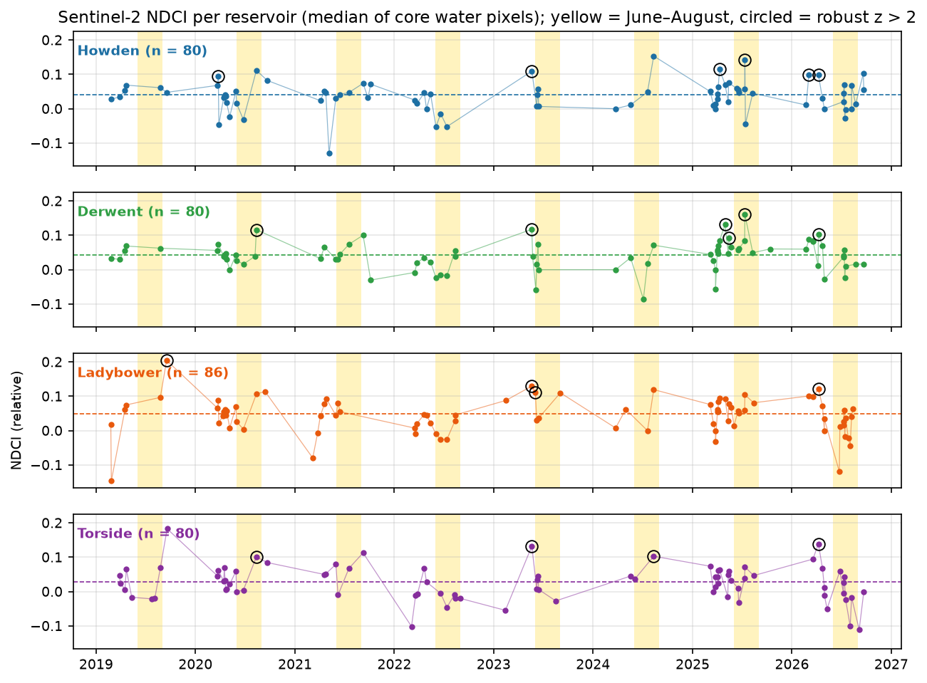
The individual dates are noisy, so it is easier to see the seasonal pattern in a monthly climatology: the median and interquartile range of each calendar month over all years.

               spring      summer     autumn
Howden     0.035 (42)  0.045 (29)  0.071 (7)
Derwent    0.044 (44)  0.038 (30)  0.038 (4)
Ladybower  0.054 (48)  0.036 (32)  0.114 (3)
Torside    0.042 (43)  0.007 (30)  0.042 (6)

             ndci     mci    ndti     red  green_blue   n
reservoir
Howden     0.0412  0.0004 -0.0308  0.0094      0.8301  80
Derwent    0.0421  0.0002 -0.0395  0.0098      0.8525  80
Ladybower  0.0490  0.0003 -0.0355  0.0096      0.8828  86
Torside    0.0287  0.0007 -0.0078  0.0098      0.8245  80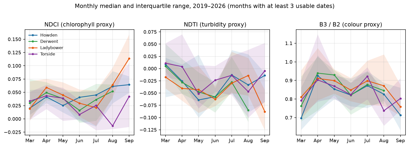

What the indices suggest, with the caveats in mind:

• Ladybower has the highest median NDCI (0.049 over 86 dates). It is the largest and lowest of the three Upper Derwent reservoirs and receives the water that has passed through Howden and Derwent.
• The Upper Derwent reservoirs show two NDCI peaks: one in April (Ladybower’s April median is 0.059) and a larger one in August and September (Ladybower 0.064 in August, 0.114 in September, though from only 3 September dates). That pattern is consistent with the classic temperate-lake cycle of a spring diatom bloom and a late-summer bloom, with a clear-water phase in between.
• Torside behaves differently. It has the lowest NDCI (0.029) and the highest turbidity proxy (NDTI −0.008, against −0.031 to −0.040 for the others), and its summer NDCI is close to zero. On the map date its north-eastern arm had exposed bed (Step 7). Shallow, drawn-down margins can stir up sediment, which would fit a more turbid, less algal signal, but the satellite alone cannot prove the cause.
• The colour ratio B3/B2 peaks in April and July. In theory, more peat colour absorbs more blue and raises B3/B2. In practice, Sen2Cor tends to over-correct the blue band over dark water, so median B3/B2 is below 1 even though the water is brown. Treat it as the weakest of the indices.

Step 6: rank the dates most worth investigating

A water manager does not need a perfect concentration every five days. They need to know which dates look unusual, so someone can check the sampling records or go out with a sonde. We compare each date with the same reservoir’s typical value for that calendar month, using a robust z-score (median and median absolute deviation). Months with fewer than five observations fall back to the whole record:

good["month"] = good["date"].dt.month
grp = good.groupby(["reservoir", "month"])["ndci"]
good["clim_med"] = grp.transform("median")
good["clim_mad"] = grp.transform(lambda x: (x - x.median()).abs().median())
good["clim_n"] = grp.transform("size")
# Months with fewer than five observations fall back to the reservoir's whole-record statistics.
whole = good.groupby("reservoir")["ndci"]
few = good["clim_n"] < 5
good.loc[few, "clim_med"] = whole.transform("median")[few]
good.loc[few, "clim_mad"] = whole.transform(lambda x: (x - x.median()).abs().median())[few]
good["ndci_z"] = (good["ndci"] - good["clim_med"]) / (1.4826 * good["clim_mad"])
# If most reservoirs spike on the same day, suspect the atmosphere (haze, aerosol model) before the water.
high = good[good["ndci_z"] > 2]
good["n_high_same_day"] = good["date"].map(high.groupby("date").size()).fillna(0).astype(int)
good["flag"] = np.where(good["n_high_same_day"] >= 3, "check atmosphere (≥3 reservoirs high)",
                        np.where(good["ndci_z"] > 2, "investigate", ""))

The last check is the most useful one. Separate reservoirs rarely bloom on exactly the same day, but an error in the atmospheric correction affects the whole scene. So when three or more reservoirs are high on the same date, the atmosphere is the first suspect.

      date reservoir  ndci  ndci_z   ndti  green_blue  sun_zenith                                  flag
2023-05-21   Derwent 0.118   4.873 -0.088       0.947        34.8 check atmosphere (≥3 reservoirs high)
2025-04-10    Howden 0.115   3.922 -0.011       1.093        46.8                           investigate
2019-09-17 Ladybower 0.205   3.484  0.000       0.660        51.9                           investigate
2025-05-13   Derwent 0.093   3.331  0.025       1.167        35.9                           investigate
2025-04-30   Derwent 0.131   3.261 -0.049       0.970        39.9                           investigate
2020-08-12   Derwent 0.116   3.181 -0.121       0.866        40.0                           investigate
2026-04-08    Howden 0.099   3.038  0.045       1.455        47.2 check atmosphere (≥3 reservoirs high)
2026-04-08   Torside 0.139   2.997  0.087       1.738        47.2 check atmosphere (≥3 reservoirs high)
2026-04-08 Ladybower 0.122   2.960  0.000       1.418        47.2 check atmosphere (≥3 reservoirs high)
2023-05-21    Howden 0.109   2.604 -0.106       0.932        34.8 check atmosphere (≥3 reservoirs high)
2026-03-04    Howden 0.098   2.602  0.150       0.515        61.1                           investigate
2025-07-12    Howden 0.143   2.576  0.069       1.373        33.0                           investigate

Spring 2025 stands out: Howden on 10 April and Derwent on 30 April and 13 May were all well above their usual April and May values, while the other reservoirs were not. That fits a real spring bloom. The two scene-wide spikes, on 21 May 2023 and 8 April 2026, are more likely to be haze or an aerosol error, though a regional bloom after a warm spell is possible. In both cases the next step is the same: look at the true-colour image and check it against sampling records.

Step 7: map NDCI and turbidity for one clear summer date

For the maps, the script chooses the summer date on which all four reservoirs had the most clear water and the least SWIR haze:

12 July 2026  S2B_MSIL2A_20260712T112109_R037_T30UWE_20260712T133747  sun zenith 33.0°
Howden     NDCI p10/median/p90  0.019  0.052  0.112 | NDTI median  0.028
Derwent    NDCI p10/median/p90  0.023  0.059  0.110 | NDTI median  0.009
Ladybower  NDCI p10/median/p90  0.023  0.056  0.100 | NDTI median  0.011
Torside    NDCI p10/median/p90  0.017  0.041  0.070 | NDTI median  0.022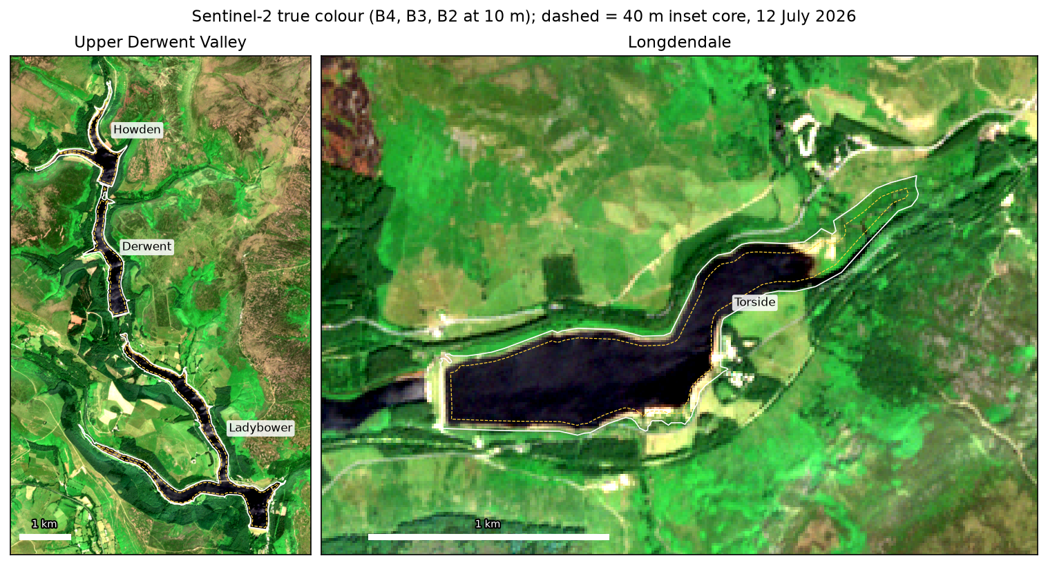

Per-pixel ratios of such dark water are noisy, so for mapping only we average the bands over 3 × 3 water pixels (60 m) before computing the indices:

def smooth(a: np.ndarray, mask: np.ndarray) -> np.ndarray:
    """3 x 3 mean over water pixels only (60 m), to tame pixel noise in very dark water."""
    v = ndimage.uniform_filter(np.where(mask, a, 0), 3)
    w = ndimage.uniform_filter(mask.astype("float32"), 3)
    with np.errstate(divide="ignore", invalid="ignore"):
        return np.where(mask, v / w, np.nan)


s = {b: smooth(r[b], water) for b in ("B03", "B04", "B05")}
with np.errstate(divide="ignore", invalid="ignore"):
    ndci_map = (s["B05"] - s["B04"]) / (s["B05"] + s["B04"])
    ndti_map = (s["B04"] - s["B03"]) / (s["B04"] + s["B03"])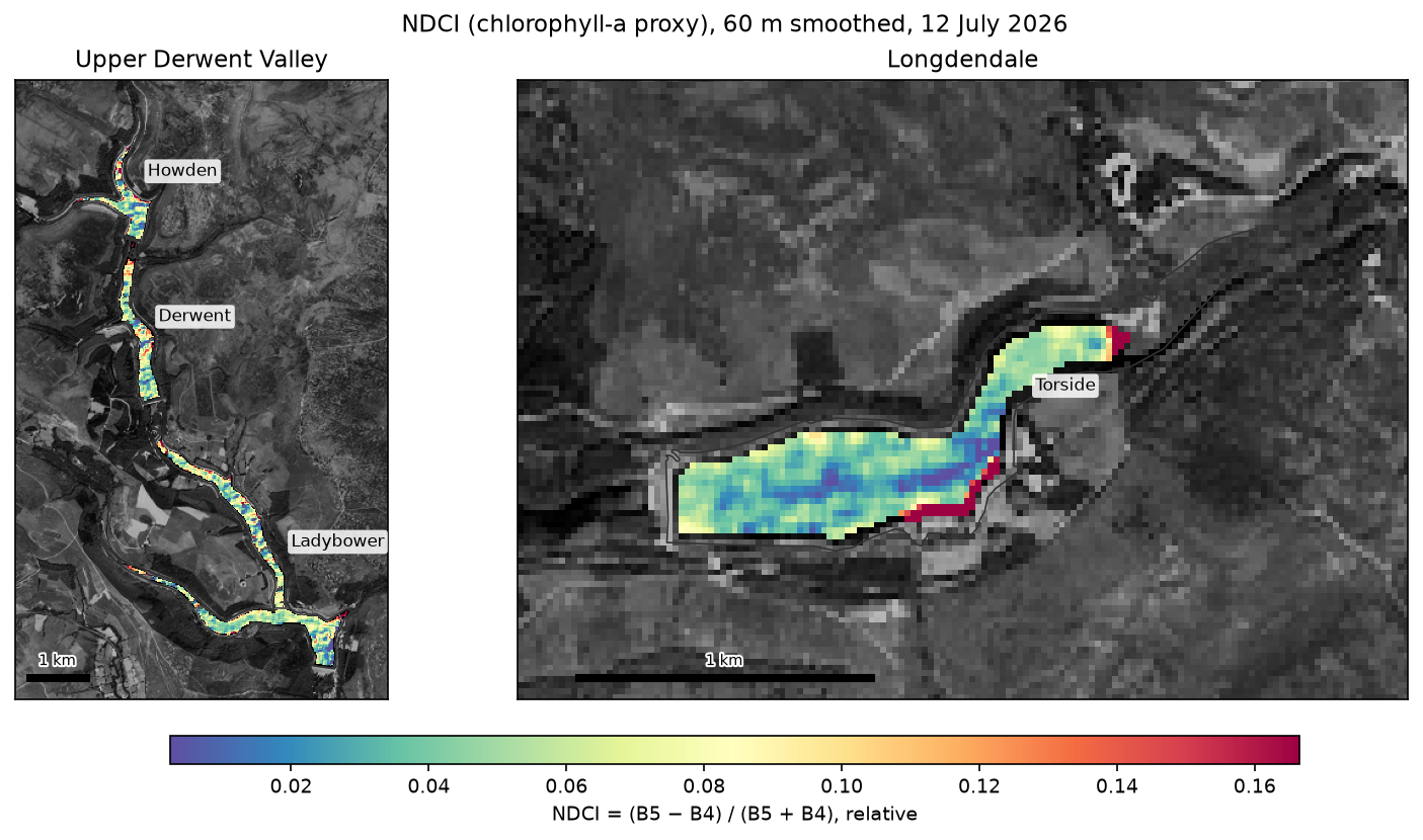

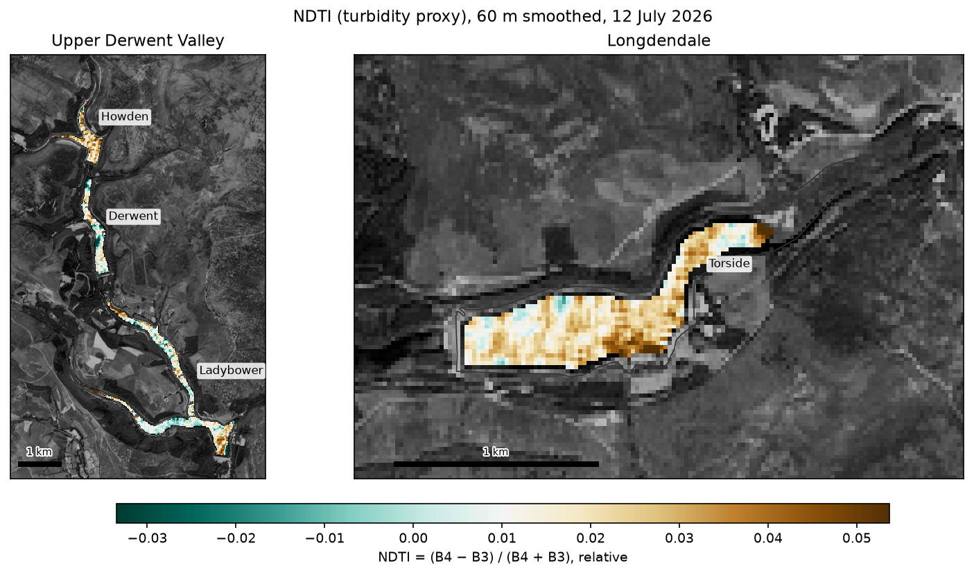
The maps show why the inset matters. Even 40 m from the shore, the pixels next to steep wooded slopes have higher NDCI than the open water. The adjacency effect (light scattered from bright land into the view of dark water) and terrain shadow both add red-edge signal that is not algae. For a reservoir only 300–400 m wide, that affects a large share of the surface.

Step 8: export a tidy CSV per reservoir

Every scene is kept in the export, with a qc column, so you can see why a date was rejected and change the thresholds later:

keep = ["date", "reservoir", "item_id", "orbit", "baseline", "sun_zenith", "clear_frac", "water_frac", "n_pixels",
        *BANDS_RHO, "ndci", "mci", "ndti", "red", "green_blue", "mndwi", "qc"]
tidy = obs[keep].merge(good[["item_id", "reservoir", "ndci_z", "flag"]], on=["item_id", "reservoir"], how="left")
for name in RESERVOIRS:
    f = OUT / f"{name.lower()}_sentinel2_water_quality.csv"
    t = tidy[tidy["reservoir"] == name]
    t.round(5).to_csv(f, index=False, date_format="%Y-%m-%d")

howden_sentinel2_water_quality.csv          821 rows,  80 usable
derwent_sentinel2_water_quality.csv         821 rows,  80 usable
ladybower_sentinel2_water_quality.csv       821 rows,  86 usable
torside_sentinel2_water_quality.csv         821 rows,  80 usable

Each row is one scene and one reservoir, with the clear and water fractions, the seven median reflectances, the indices, the quality label and, for usable dates, the robust z-score and flag. The files load straight into pandas, R, Excel or a dashboard.

Step 9: check against Environment Agency samples

Most routine monitoring of these reservoirs is done by the water companies: Severn Trent for the Upper Derwent and United Utilities for Longdendale. Their operational data is not published. However, the Environment Agency Water Quality Archive is public and has an open API. Searching it found sampling points at all four reservoirs, with chlorophyll-a and colour:

EA = "https://environment.data.gov.uk/water-quality"
POINTS = {"MD-49714900": "Howden", "MD-49714220": "Derwent", "MD-LSN0395": "Ladybower", "NW-88021743": "Torside"}
DETERMINANDS = {"7887": "chlorophyll_ugl", "0072": "colour_hazen"}

resp = requests.get(f"{EA}/sampling-point/{point}/observation", headers={"Accept": "text/csv"},
                    params={"dateFrom": "2019-01-01", "dateTo": "2026-10-14", "determinand": code,
                            "limit": 250, "skip": skip}, timeout=60)

reservoir             var  n        min        max
  Derwent chlorophyll_ugl 47 2019-01-16 2026-08-13
  Derwent    colour_hazen 19 2019-01-16 2022-07-19
   Howden chlorophyll_ugl 11 2019-01-16 2020-03-19
   Howden    colour_hazen 11 2019-01-16 2020-03-19
Ladybower chlorophyll_ugl  5 2026-04-20 2026-08-05
Ladybower    colour_hazen  5 2026-04-20 2026-08-05
  Torside chlorophyll_ugl 15 2019-02-11 2020-03-18
  Torside    colour_hazen 15 2019-02-11 2020-03-18

We pair each sample with the nearest usable Sentinel-2 date within ±3 days. Values below the detection limit, such as <0.5, are kept at the limit and marked:

reservoir sample_date    s2_date  value  censored    ndci     mci
   Howden  2019-02-21 2019-02-24   0.50      True  0.0279  0.0023
   Howden  2019-03-25 2019-03-28   0.60     False  0.0340  0.0012
   Howden  2020-03-19 2020-03-22   0.50      True  0.0680  0.0006
  Derwent  2019-02-21 2019-02-24   0.50      True  0.0333  0.0025
  Derwent  2019-03-25 2019-03-28   0.50      True  0.0299  0.0011
  Derwent  2021-06-18 2021-06-15   3.00     False  0.0451 -0.0004
  Derwent  2022-04-20 2022-04-21   0.76     False  0.0352  0.0002
  Derwent  2022-06-23 2022-06-20   8.70     False -0.0145  0.0013
  Derwent  2022-08-10 2022-08-12   1.80     False  0.0548  0.0017
  Derwent  2024-03-21 2024-03-24   0.59     False  0.0000  0.0004
  Derwent  2025-05-15 2025-05-13   1.70     False  0.0925  0.0001
  Derwent  2025-06-17 2025-06-17   1.30     False  0.0571  0.0004
  Derwent  2026-04-21 2026-04-23   1.40     False  0.0704 -0.0005
Ladybower  2026-04-20 2026-04-23   1.80     False  0.0714 -0.0008
Ladybower  2026-07-10 2026-07-09   4.50     False  0.0159  0.0010
Ladybower  2026-08-05 2026-08-03   9.00     False -0.0435  0.0013
  Torside  2019-04-24 2019-04-22   2.70     False  0.0649 -0.0000
  Torside  2019-08-28 2019-08-25   5.00     False  0.0687 -0.0001
chlorophyll vs NDCI    n = 18  Spearman rho = -0.03  p = 0.90
chlorophyll vs MCI     n = 18  Spearman rho = -0.27  p = 0.28
colour vs B3/B2        n = 12  Spearman rho = -0.04  p = 0.91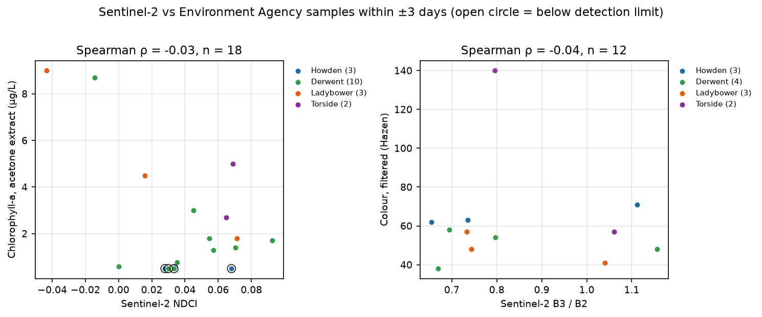

The honest result: at these reservoirs, Sentinel-2 NDCI from Sen2Cor reflectance does not track measured chlorophyll. The two highest samples, 8.7 µg/L at Derwent on 23 June 2022 and 9.0 µg/L at Ladybower on 5 August 2026, came with some of the lowest NDCI values. There are several reasons:

• The chlorophyll is low. Every sample is between 0.5 and 9 µg/L. NDCI was developed for productive, turbid water, and its red-edge peak only becomes clear above roughly 10–20 µg/L. Below that, peat colour and residual atmospheric error control the signal.
• The water is very dark. With B4 and B5 near 0.005–0.01, an atmospheric-correction error of 0.002 changes NDCI by more than the whole seasonal range.
• Small, uneven samples. There are only 18 pairs, the samples are taken at the dam or a jetty rather than the open water, and ±3 days is long enough for a bloom to move or die back.

That does not make the workflow useless. It shows what the indices can and cannot do. With this level of correction, use them to find unusual dates and spatial patterns that deserve a closer look, and keep the time series as a consistent record you can calibrate later. Do not report them as concentrations.

Pitfalls and limitations

• Relative, not calibrated. NDCI, MCI, NDTI and B3/B2 are proxies. Turning them into µg/L or NTU needs a local regression against matched samples, and the result above shows that would not work yet with Sen2Cor reflectance.
• Atmospheric correction. Sen2Cor is designed for land. Over dark water it often over-corrects the blue band and leaves errors of a few thousandths in reflectance, which is a large share of the water signal. The standard next steps are ACOLITE (dark spectrum fitting) or C2RCC in ESA SNAP, both made for inland and coastal water, run on Level-1C data.
• Cloud and shadow. About 82% of reservoir-dates were lost. Shadows from small cumulus clouds that SCL misses are a common cause of false dark or bright water; the 100 m cloud buffer helps but is not perfect.
• Adjacency and terrain shadow. In narrow valleys, scattered light from bright land and shadows from steep slopes reach well beyond 40 m, as the NDCI map at Torside shows. A 60–100 m inset or an adjacency correction (ACOLITE has one) is safer for science-grade work.
• Sunglint. In summer the sun is high and wind-roughened water can reflect sunlight straight towards the sensor. The SWIR test (median B11 above 0.03) catches strong glint, but weak glint still lifts all bands.
• Shallow water and drawdown. In shallow margins and during low water, the bed contributes to the signal. The NIR test removes exposed mud, but not water a few tens of centimetres deep over a bright bed.
• Peat colour (CDOM). Brown water absorbs blue and green strongly and lowers the signal in every band, which leaves less room for the chlorophyll signal. The colour ratio is unreliable while the blue band is poorly corrected.
• Low winter sun. Above a solar zenith angle of 70° the atmospheric path is long and the signal weak, so winter has almost no data.

Frequently asked questions

Can Sentinel-2 measure chlorophyll?

Not directly. Sentinel-2 measures reflected light, and its red-edge band B5 (705 nm) responds to chlorophyll, so indices such as NDCI and MCI give a chlorophyll proxy. In productive, turbid lakes with tens of µg/L, published algorithms calibrated with field samples can estimate concentrations reasonably well. In clear or peat-stained water with low chlorophyll, such as these Peak District reservoirs, the signal is too weak for reliable estimates without water-specific atmospheric correction and local calibration.

How do you monitor algal blooms from satellite?

Use a sensor with a red-edge band (Sentinel-2 MSI or Sentinel-3 OLCI), mask cloud and shoreline pixels, compute a chlorophyll index such as NDCI, MCI or, with OLCI, the cyanobacteria index, and compare each date with that lake’s own seasonal normal. Treat large anomalies as alerts to investigate with sampling, as in Step 6. For larger lakes, the Copernicus Land Monitoring Service publishes ready-made lake water-quality products such as turbidity and trophic state.

What is NDCI?

The Normalised Difference Chlorophyll Index, (B5 − B4) / (B5 + B4) for Sentinel-2, was published by Mishra and Mishra in 2012. Chlorophyll absorbs red light (B4, 665 nm), while algal cells reflect strongly just beyond the absorption, near 705 nm (B5). More algae push NDCI up. Values are relative and depend on the atmospheric correction.

Which satellite is best for monitoring small reservoirs?

Sentinel-2 is the best free option for reservoirs smaller than a few square kilometres, with 10–20 m pixels, a red-edge band and a 2–5 day revisit. Landsat 8 and 9 have 30 m pixels and no red-edge band, so they suit turbidity and temperature rather than chlorophyll. Sentinel-3 OLCI has excellent water bands but 300 m pixels, which is too coarse for lakes narrower than about 1 km. Commercial sensors such as PlanetScope have more frequent images but weaker spectral and radiometric quality.

Why is my reservoir’s MNDWI negative?

Very dark water, such as peat-stained upland reservoirs, reflects only about 1% of green light. After atmospheric correction, the residual signal in the SWIR band can be just as large, so MNDWI is close to zero or negative. Use a known outline shrunk inwards, the SCL cloud mask and a near-infrared threshold instead, as in Step 3.

Is there public water quality data for UK reservoirs?

Partly. The Environment Agency Water Quality Archive is open and includes some reservoir samples, as used in Step 9. Most operational monitoring of drinking-water reservoirs is done by the water companies and is not published. The UK Centre for Ecology & Hydrology runs long-term monitoring at some lakes, mainly in Cumbria and Scotland.

Next steps

• Process Level-1C scenes with ACOLITE or C2RCC and rerun the comparison with the Environment Agency samples; a water-specific correction is the single biggest improvement.
• Add Sentinel-3 OLCI for a large lake nearby, or switch to a larger lake such as Rutland Water, where 300 m pixels are usable.
• Add Landsat 8 and 9 to fill gaps in the turbidity record, after harmonising the bands.
• Map the reservoirs’ water area through the year, as in Measuring Lake Mead’s shrinking shoreline with Sentinel-2 and STAC or our earlier Lake Mead drought post.
• When cloud blocks every optical image, track water extent with radar instead: Sentinel-1 SAR flood mapping in Python.
• Get the inflowing streams and catchments with OSMnx or OS Open Rivers, and relate the colour signal to peat cover upstream.

Data and licences

• Sentinel-2 L2A: contains modified Copernicus Sentinel data 2019–2026, processed by ESA. Accessed as Cloud Optimised GeoTIFFs from the Microsoft Planetary Computer on 15 October 2026.
• Reservoir outlines: © OpenStreetMap contributors, available under the Open Database Licence (ODbL).
• Water quality samples: Environment Agency Water Quality Archive, © Environment Agency, licensed under the Open Government Licence v3.0. Accessed on 15 October 2026.
• Country outlines: Natural Earth, public domain.
• References: Mishra, S. and Mishra, D. R. (2012), “Normalized difference chlorophyll index”, Remote Sensing of Environment 117; Gower, J. et al. (2005), “Detection of intense plankton blooms using the 709 nm band of the MERIS imaging spectrometer”, International Journal of Remote Sensing 26(9); Lacaux, J. P. et al. (2007), Remote Sensing of Environment 106(1).
• Code: reservoir_water_quality.py, tested with Python 3.12.0, pystac-client 0.9.0, planetary-computer 1.0.0, rasterio 1.5.2, osmnx 2.1.1 and pandas 3.0.6.