Sentinel-1 SAR flood mapping in Python: the 2022 Pakistan floods

Short answer: to map a flood with Sentinel-1 in Python, load a radar image from before the flood and one from during it, convert the VV backscatter to decibels (10 * log10), reduce speckle with a filter such as Lee, and choose a water threshold automatically with Otsu’s method (skimage.filters.threshold_otsu). Pixels below the threshold are open water. Pixels that are water now but were not before are flood. Multiply the count by the pixel area to get the flooded area.

In August and September 2022, record monsoon rain and glacier melt put about a third of Pakistan under water. Over 1,700 people died and more than 30 million were affected. Cloud covered Sindh for weeks, which made optical satellites such as Sentinel-2 almost useless. Radar sees through cloud. In this tutorial we use free Sentinel-1 data to map the flood around Manchar Lake and the town of Dadu, and we follow it from June to December.

You will learn how to:

1. search the Microsoft Planetary Computer’s Sentinel-1 RTC collection with pystac-client, and why you should stick to one orbit;
2. convert backscatter to decibels, and why you average in linear power;
3. reduce speckle with a Lee filter written in a few lines of NumPy and SciPy;
4. pick a water threshold automatically with Otsu’s method;
5. turn the result into flood extent maps, areas, a GeoTIFF and a GeoPackage, and a time series for the whole monsoon.

All outputs below are real results from sar_flood_mapping.py, run on 15 October 2026 with Python 3.12, pystac-client 0.9.0 and rasterio 1.5.2.

Why radar for floods?

Sentinel-1 carries a C-band synthetic aperture radar (SAR). It sends microwave pulses obliquely towards the ground and records how much energy comes back: the backscatter. Rough surfaces such as fields, towns and trees scatter energy in all directions, so some returns to the satellite and they look bright. Calm open water acts like a mirror and reflects the pulse away, so it looks very dark. Because the radar makes its own illumination at a wavelength of 5.6 cm, it works at night and through cloud and rain.

We use the VV polarisation (vertical transmit, vertical receive), which gives the clearest contrast between water and land. Sentinel-1 also records VH, which helps with vegetation.

Step 1: search for Sentinel-1 RTC scenes with STAC

The Planetary Computer’s sentinel-1-rtc collection holds Sentinel-1 GRD scenes that have already been radiometrically terrain corrected (RTC): geocoded to a map grid and corrected for slope brightness, as Cloud Optimised GeoTIFFs. Doing that yourself from raw GRD data is a job for ESA SNAP or sarsen.

Different orbits look at the ground from different angles, which changes the backscatter. So we keep one relative orbit (42, ascending) and compare like with like:

STAC_URL = "https://planetarycomputer.microsoft.com/api/stac/v1"
BBOX = (67.45, 26.15, 68.25, 27.05)  # lon/lat: Manchar Lake, Dadu and the Indus in Sindh, Pakistan
SEASON = "2022-06-01/2022-12-31"
ORBIT = 42                            # one relative orbit = identical viewing geometry on every date
BEFORE, AFTER = "2022-06-16", "2022-09-08"
RES = 40                              # analysis resolution in metres
CRS = "EPSG:32642"                    # UTM zone 42N, the native CRS of these scenes

catalog = pystac_client.Client.open(STAC_URL, modifier=planetary_computer.sign_inplace)
search = catalog.search(collections=["sentinel-1-rtc"], bbox=BBOX, datetime=SEASON,
                        query={"sat:relative_orbit": {"eq": ORBIT}, "sat:orbit_state": {"eq": "ascending"}})
items = sorted(search.items(), key=lambda i: i.datetime)

planetary_computer.sign_inplace adds a free, short-lived access token to every asset URL; no account is needed.

18 scenes from relative orbit 42 (ascending), 04 Jun to 25 Dec 2022
S1A_IW_GRDH_1SDV_20220908T133610_20220908T133635_044914_055D60_rtc
assets: vh, vv, tilejson, rendered_preview
polarisations: ['VV', 'VH'] | mode IW | pixel 10 m | ENL 4.4 | EPSG:32642
vv raster:bands: [{'nodata': -32768, 'data_type': 'float32', 'spatial_resolution': 10}]

That is one scene every 12 days. Sentinel-1B failed in December 2021, so in 2022 only Sentinel-1A was flying. Since Sentinel-1C began operations in 2025, the revisit is back to 6 days. The sar:looks_equivalent_number property (ENL 4.4) tells us how much the speckle has already been averaged down. We use it in the filter below.

Step 2: understand decibels and speckle

The RTC values are linear power (γ⁰). Water is around 0.001–0.01 and a bright building can exceed 10. That range is too wide to see or threshold, so we convert to decibels:

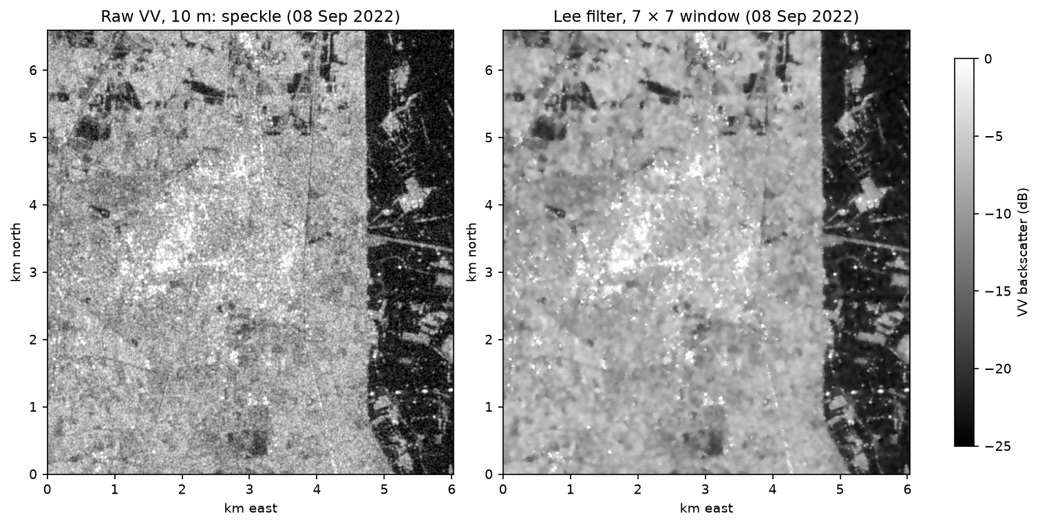
def to_db(power: np.ndarray) -> np.ndarray:
    with np.errstate(divide="ignore", invalid="ignore"):
        return 10 * np.log10(np.where(power > 0, power, np.nan))

Every SAR image also has speckle, a grainy texture from interference between the many scatterers in each pixel. It is not sensor noise you can calibrate away; it is part of how coherent imaging works. The Lee filter (Lee, 1980) smooths homogeneous areas while keeping edges. It compares the local variance with the variance expected from speckle alone (1 / ENL), and smooths only where the two are similar:

def lee_filter(img: np.ndarray, size: int = 7, enl: float = 4.4) -> np.ndarray:
    """Lee (1980) speckle filter on linear power. enl = equivalent number of looks."""
    nan = np.isnan(img)
    img = np.where(nan, np.nanmedian(img), img)
    mean = ndimage.uniform_filter(img, size)
    var = np.maximum(ndimage.uniform_filter(img * img, size) - mean * mean, 0)
    ci2 = var / np.maximum(mean * mean, 1e-12)        # local coefficient of variation, squared
    w = np.clip(1 - (1 / enl) / np.maximum(ci2, 1e-12), 0, 1)
    out = mean + w * (img - mean)                      # smooth flat areas, keep edges
    out[nan] = np.nan
    return out

To see what it does, we read a 6 km chip around Dadu at the full 10 m resolution, using a rasterio window so only that part of the COG is downloaded:

CHIP = (67.75, 26.70, 67.81, 26.76)  # 6 km box around Dadu town and the floodwater surrounding it
cx, cy = to_utm.transform([CHIP[0], CHIP[2]], [CHIP[1], CHIP[3]])
with rasterio.open(example.assets["vv"].href) as src:
    chip = src.read(1, window=from_bounds(cx[0], cy[0], cx[1], cy[1], src.transform)).astype("float32")
chip[chip == -32768] = np.nan
chip_lee = lee_filter(chip, size=7, enl=ENL)


def local_std(db: np.ndarray, size: int = 5) -> float:
    """Median of the 5 x 5 moving-window standard deviation: pixel-to-pixel noise, not scene contrast."""
    m = ndimage.uniform_filter(db, size)
    return float(np.nanmedian(np.sqrt(np.maximum(ndimage.uniform_filter(db * db, size) - m * m, 0))))


print(f"pixel-to-pixel noise (median 5x5 std): raw {local_std(to_db(chip)):.2f} dB, Lee {local_std(to_db(chip_lee)):.2f} dB")

chip 603 x 659 pixels; linear gamma0 0.0009..30.54
pixel-to-pixel noise (median 5x5 std): raw 1.84 dB, Lee 0.65 dB

The filter cuts the pixel-to-pixel variation from 1.84 dB to 0.65 dB, while the edges of the town, fields and floodwater stay sharp.

Step 3: read every date onto one 40 m grid

As in the Sentinel-2 Lake Mead tutorial, rasterio’s WarpedVRT streams each COG straight onto a fixed grid, reading from the internal overviews so only a fraction of the data is downloaded. Our study area is 81 × 100 km, and 40 m pixels are plenty for a flood of this size.

def read_gamma0(href: str) -> np.ndarray:
    """Warp a remote RTC COG onto the analysis grid (averaging linear power), NaN where empty."""
    with rasterio.open(href) as src, WarpedVRT(src, crs=CRS, transform=TRANSFORM, width=WIDTH, height=HEIGHT,
                                               resampling=Resampling.average, src_nodata=src.nodata,
                                               nodata=np.nan, dtype="float32") as vrt:
        return vrt.read(1)


vv_db = {}
for it in items:
    d = it.datetime.strftime("%Y-%m-%d")
    power = read_gamma0(it.assets["vv"].href)
    # Each 40 m pixel averages 16 pixels (~4 independent resolution cells), so ENL rises ~4x.
    vv_db[d] = to_db(lee_filter(power, size=5, enl=ENL * 4))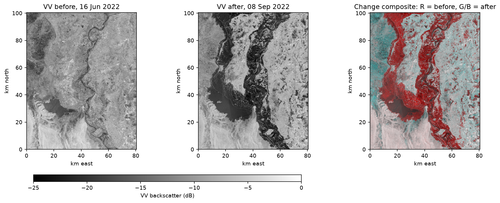

The composite on the right is a quick, threshold-free way to see change: areas that stayed the same are grey, and areas that went dark are red.

Step 4: choose the water threshold with Otsu’s method

The histogram of the flood image has two peaks: water near −20 dB and land near −8 dB. Otsu’s method finds the threshold that best separates them, by maximising the variance between the two classes:

before, after = vv_db[BEFORE], vv_db[AFTER]
valid = np.isfinite(before) & np.isfinite(after)
thr = threshold_otsu(after[valid])

VV threshold from 2022-09-08: -14.1 dB
median VV: water-side -19.8 dB, land-side -8.3 dB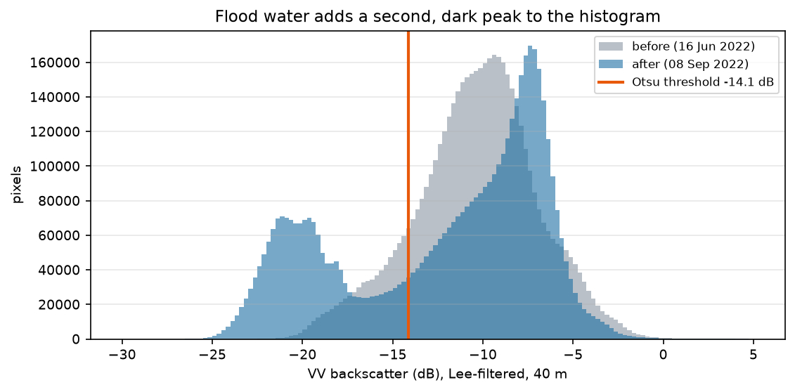

The threshold comes from the flood image, where water is plentiful. We apply it to every date, so all dates are classified the same way. Commonly published thresholds for VV water are around −15 to −18 dB, so −14.1 dB is in the expected range for a scene with this much water.

Step 5: build a clean water mask and the flood extent

A raw threshold leaves single dark pixels everywhere: radar shadow, smooth roads and tarmac. A morphological opening removes isolated pixels, and a minimum patch size of 7 pixels (about 1 ha) removes small speckles:

def water_mask(db: np.ndarray) -> np.ndarray:
    w = np.isfinite(db) & (db < thr)
    w = ndimage.binary_opening(w, iterations=1)                  # drop isolated dark pixels
    lab, n = ndimage.label(w)
    sizes = ndimage.sum(w, lab, index=np.arange(1, n + 1))
    return np.isin(lab, 1 + np.flatnonzero(sizes >= 7))          # keep patches >= ~1 ha


water_before, water_after = water_mask(before) & valid, water_mask(after) & valid
flood = water_after & ~water_before

Flood = water now that was not water before. Comparing with a pre-flood image removes permanent water, such as Manchar Lake and the Indus channel. It also removes surfaces that are always dark, such as smooth sand or tarmac.

valid area: 8,095 km²
water on 2022-06-16: 958 km²
water on 2022-09-08: 2,470 km²
newly flooded: 1,933 km² (23.9% of the area)
water before but not after: 421 km²
pixels at least 3 dB darker: 2,432 km²; of the Otsu flood pixels, 97% dropped by 3 dB or more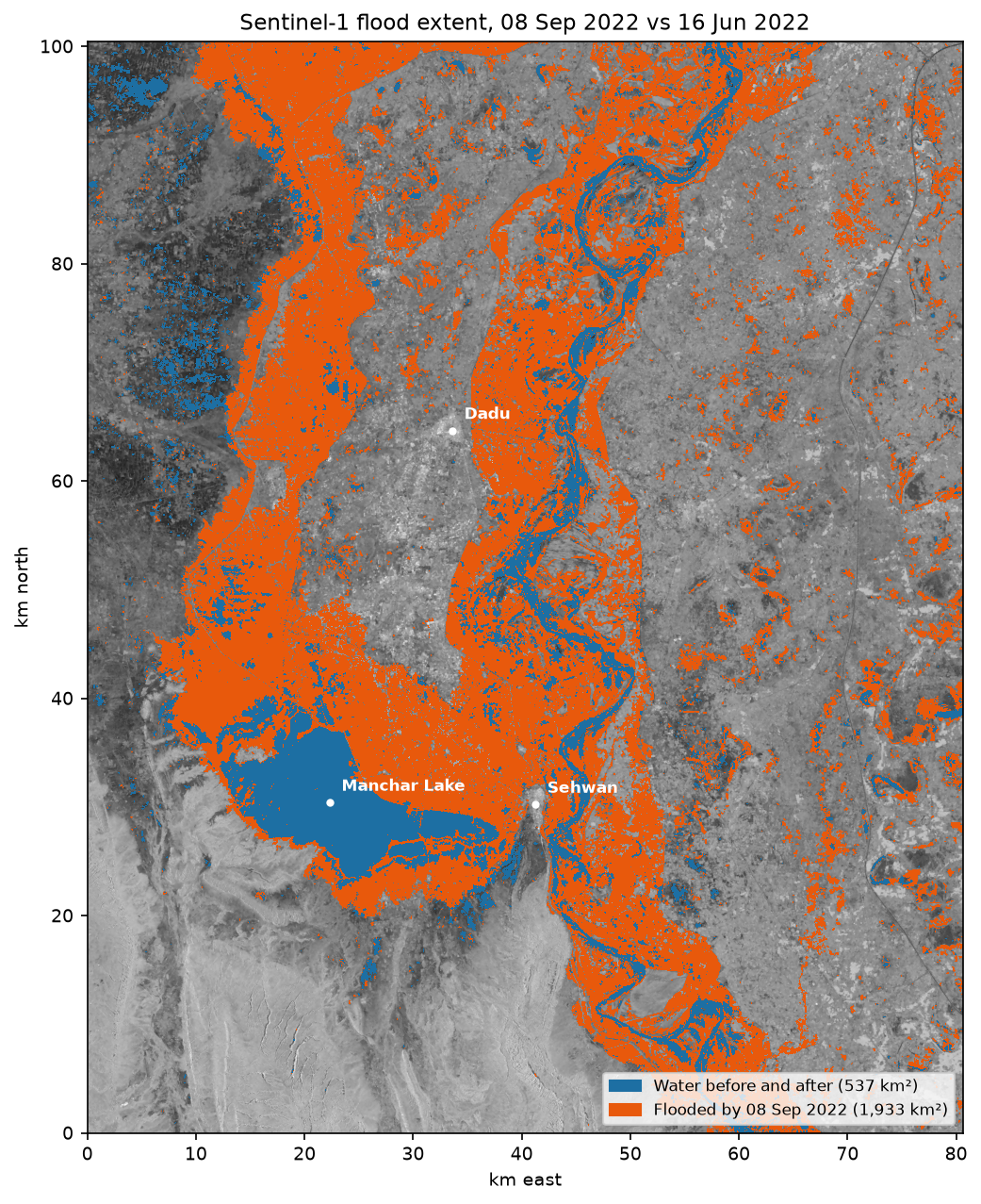

Two checks give confidence in the result:

• A threshold-free cross-check. 97% of the flood pixels became at least 3 dB darker, which is the classic change-detection criterion.
• Lost water is plausible. 421 km² was water in June but not in September. Some of it is seasonal water that drained or was replaced by growing crops. Some is probably flooded vegetation, which looks bright rather than dark (see the limitations below).

Finally, save the result as a classified GeoTIFF and as vector polygons for use in QGIS or a web map:

shapes = rasterio.features.shapes(flood.astype("uint8"), mask=flood, transform=TRANSFORM)
polys = gpd.GeoDataFrame.from_features([{"geometry": g, "properties": {"class": "flood"}} for g, _ in shapes],
                                       crs=CRS)
polys["area_km2"] = polys.area / 1e6
polys.to_file(OUT / "flood_extent_2022-09-08.gpkg", driver="GPKG")

8,320 flood polygons, total 1,933 km², largest 1,208 km²

Step 6: follow the flood through time

Because every scene is on the same grid, a time series is just a loop:

rows = []
for d in dates:
    v = np.isfinite(vv_db[d]) & valid
    w = water_mask(vv_db[d]) & v
    rows.append({"date": pd.Timestamp(d), "water_km2": round(w.sum() * PIXEL_KM2),
                 "flooded_km2": round((w & ~water_before).sum() * PIXEL_KM2), "valid_pct": round(v.mean() * 100, 1)})
ts = pd.DataFrame(rows)

      date  water_km2  flooded_km2  valid_pct
2022-06-04        925           89      100.0
2022-06-16        958            0      100.0
2022-06-28       1065          162      100.0
2022-07-10        767          150      100.0
2022-07-22       1012          374      100.0
2022-08-03       1191          562      100.0
2022-08-15        912          490      100.0
2022-08-27       2156         1608      100.0
2022-09-08       2470         1933      100.0
2022-09-20       1807         1369      100.0
2022-10-02       1428         1022      100.0
2022-10-14       1281          872      100.0
2022-10-26       1112          713      100.0
2022-11-07        985          586      100.0
2022-11-19        874          482      100.0
2022-12-01        816          419      100.0
2022-12-13        768          366      100.0
2022-12-25        758          332      100.0
peak: 08 September 2022, 1,933 km² newly flooded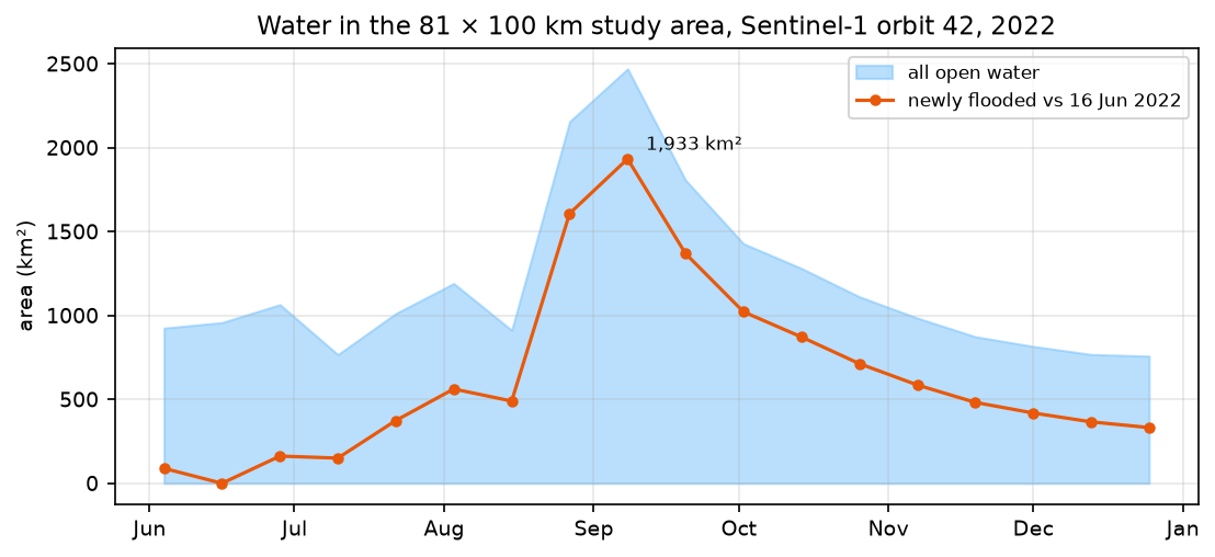

The curve tells the story of the disaster. Rain in July and early August flooded fields locally. The main flood wave arrived in late August, as the Indus and hill torrents from the west filled the plain. In early September, the authorities breached the embankment of Manchar Lake to protect the towns of Sehwan and Bhan Saeedabad, and the water drained only slowly through the autumn. Months later, land that should have been sown with wheat was still under water.

Limitations and how to improve them

• Dark is not always water. Smooth tarmac, dry sand and radar shadow behind hills are dark too. Change detection removes most of these; a HAND (height above nearest drainage) or slope mask from the Copernicus DEM removes the rest.
• Wind roughens water. Strong wind can make a lake look bright and be missed.
• Flooded vegetation and towns look bright, not dark. Radar bounces between the water surface and stems or walls (double bounce), so flooded crops, forest and streets are under-mapped by a darkness threshold. VH and the VV/VH ratio help.
• One threshold for a huge area can be biased. Use tiled Otsu, or validate against a Copernicus Emergency Management Service map of the same event.

Frequently asked questions

Can Sentinel-1 see through clouds?

Yes. Sentinel-1 is a C-band radar with a 5.6 cm wavelength, which passes through cloud, haze and smoke, and it makes its own illumination, so it works at night too. Only very heavy rain cells cause minor effects. That is why it is the standard satellite for flood mapping.

What dB threshold should I use for water in Sentinel-1?

There is no universal value. Open water in VV is usually below about −15 to −18 dB, and in VH below about −22 to −25 dB, but it depends on wind, incidence angle and processing. Compute the threshold from your own image with Otsu’s method or a tiled variant, as in this tutorial, rather than copying a number.

What is the difference between Sentinel-1 GRD and RTC?

GRD (Ground Range Detected) is ESA’s standard product: calibrated backscatter in the radar’s own ground-range geometry, projected onto an Earth ellipsoid without terrain correction. RTC (radiometrically terrain corrected) is GRD that has also been geocoded with a DEM and corrected for the brightening and darkening of slopes. For flood mapping in hilly areas, use RTC; on a flat plain like Sindh, GRD is very similar.

Why is my SAR image so grainy?

That is speckle, a feature of every coherent radar image. Reduce it with a speckle filter (Lee, refined Lee, Gamma-MAP), by averaging pixels (multilooking), or by averaging several dates. Filter the linear power values, not the decibels.

Is Sentinel-1 data free?

Yes. All Sentinel data is free and open under the Copernicus licence. You can download it from the Copernicus Data Space Ecosystem, from ASF, or stream analysis-ready RTC from the Microsoft Planetary Computer as in this tutorial.

Next steps

• Add VH and map flooded vegetation with the VV/VH ratio.
• Mask steep and high ground with HAND computed from the Copernicus DEM; Terrain analysis in Python with rasterio and rioxarray shows how to stream and process it.
• Compare with optical water indices in Measuring Lake Mead’s shrinking shoreline with Sentinel-2 and STAC, or combine both on cloud-free days.
• Go beyond water extent to water quality in Monitoring reservoir water quality from space with Sentinel-2.- Map elevation in 3D with lidar in LiDAR point clouds in Python with laspy.
• Overlay the flood polygons on settlements and roads from OSMnx to estimate exposure.

Data and licences

• Sentinel-1 RTC: contains modified Copernicus Sentinel data 2022, processed by ESA; radiometric terrain correction by Catalyst/Microsoft. Licensed CC BY 4.0. Accessed from the Microsoft Planetary Computer on 15 October 2026.
• Reference: Lee, J.-S. (1980), “Digital image enhancement and noise filtering by use of local statistics”, IEEE Transactions on Pattern Analysis and Machine Intelligence 2(2); Otsu, N. (1979), IEEE Transactions on Systems, Man, and Cybernetics 9(1).
• Code: sar_flood_mapping.py, tested with Python 3.12.0, pystac-client 0.9.0, planetary-computer 1.0.0, rasterio 1.5.2, scipy 1.18.1 and scikit-image 0.26.0.