LiDAR point clouds in Python with laspy: from a LAZ file to a DTM, DSM and canopy height model

Short answer: to work with lidar in Python, pip install "laspy[lazrs]", then las = laspy.read("file.laz") gives you NumPy arrays of x, y, z, classification and every other point attribute. A DSM is the highest point in each grid cell. A DTM is the average of the ground-classified points (class 2), with gaps interpolated. A canopy height model is DSM − DTM wherever there are trees. The rest of this tutorial does exactly that on real data, with no PDAL or GDAL command line needed.

We use free USGS 3DEP lidar of the National Mall in Washington, D.C. That gives us an independent check on the results: the Washington Monument has a surveyed height of 169.046 m.

You will learn how to:

1. find lidar tiles in a STAC catalogue and stream just your area from COPC files with laspy.CopcReader;
2. read, inspect and write LAZ files, and process big files in chunks;
3. understand classification codes, including the overlap classes that trip people up;
4. remove noise with statistical outlier removal;
5. grid the points into a 1 m DTM, DSM, normalised DSM and canopy height model, and save them as GeoTIFFs.

All outputs below are real results from lidar_dtm_chm.py, run on 15 October 2026 with Python 3.12, laspy 2.7.0 and lazrs 0.8.2.

LiDAR, LAS, LAZ and COPC in one minute

An airborne lidar scanner fires hundreds of thousands of laser pulses per second and records each echo (a return) as a 3D point. A pulse that hits a roof gives one return. A pulse that passes through a tree crown can give several: the top of the canopy, branches and finally the ground. That difference is what lets us separate trees from buildings later.

Points are stored in the LAS format, or compressed as LAZ. COPC is a LAZ file arranged as a spatial index (an octree), so you can request one city block from a 200 MB file on a server without downloading the rest. It does for point clouds what Cloud Optimised GeoTIFFs did for rasters.

Step 1: find the lidar tiles with STAC

The Microsoft Planetary Computer publishes the whole 3DEP archive as COPC in the 3dep-lidar-copc collection. We define a 1000 × 800 m box around the Washington Monument in the lidar’s own coordinate system, NAD83 / UTM zone 18N (EPSG:26918), and search the catalogue with its corners in longitude and latitude:

LON, LAT = -77.0353, 38.8895  # Washington Monument
EPSG = 26918                  # NAD83 / UTM zone 18N, the CRS of this lidar project
to_utm = Transformer.from_crs(4326, EPSG, always_xy=True)
to_ll = Transformer.from_crs(EPSG, 4326, always_xy=True)
mx, my = to_utm.transform(LON, LAT)
xmin, xmax, ymin, ymax = mx - 500, mx + 500, my - 400, my + 400
lon0, lat0 = to_ll.transform(xmin, ymin)
lon1, lat1 = to_ll.transform(xmax, ymax)

catalog = pystac_client.Client.open("https://planetarycomputer.microsoft.com/api/stac/v1",
                                    modifier=planetary_computer.sign_inplace)
items = list(catalog.search(collections=["3dep-lidar-copc"], bbox=[lon0, lat0, lon1, lat1]).items())

planetary_computer.sign_inplace adds a short-lived access token to each asset URL. It is free and needs no account.

area of interest: 1000 m x 800 m centred on the Washington Monument
USGS_LPC_MD_VA_Sandy_NCR_2014_18SUJ324306_LAS_2015  points=18,237,018
USGS_LPC_MD_VA_Sandy_NCR_2014_18SUJ324305_LAS_2015  points=13,976,445
USGS_LPC_MD_VA_Sandy_NCR_2014_18SUJ322306_LAS_2015  points=16,107,898
USGS_LPC_MD_VA_Sandy_NCR_2014_18SUJ322305_LAS_2015  points=13,997,484

The four tiles hold 62 million points between them. We only need about a tenth of those.

Step 2: stream only your area with CopcReader

laspy.CopcReader.query() takes a laspy.Bounds and fetches only the octree nodes that intersect it, using HTTP range requests:

bounds = laspy.Bounds(mins=np.array([xmin, ymin]), maxs=np.array([xmax, ymax]))
parts, header = [], None
for it in items:
    with laspy.CopcReader.open(it.assets["data"].href) as reader:
        if header is None:
            header = reader.header
        pts = reader.query(bounds)
        if len(pts):
            parts.append(pts)

LAS 1.4, point format 6, CRS: NAD83 / UTM zone 18N + NAVD88 height
18SUJ324306_LAS_2015: 0 points in the area of interest
18SUJ324305_LAS_2015: 0 points in the area of interest
18SUJ322306_LAS_2015: 2,705,087 points in the area of interest
18SUJ322305_LAS_2015: 3,449,342 points in the area of interest
streamed in 15.0 s
wrote data/national_mall.laz (27.3 MB)

The two eastern tiles overlap the longitude/latitude search rectangle but not the UTM box itself, so they return nothing. To merge the parts into one file, we create a new header and copy the attributes across. Each source tile has its own scale and offset (LAS stores coordinates as scaled integers), so copy the real-world x, y and z, not the raw X, Y and Z integers:

out_header = laspy.LasHeader(point_format=header.point_format.id, version=header.version)
out_header.offsets = np.array([xmin, ymin, 0.0])
out_header.scales = np.array([0.01, 0.01, 0.01])
out_header.add_crs(header.parse_crs())
merged = laspy.LasData(out_header)
merged.points = laspy.ScaleAwarePointRecord.zeros(sum(len(p) for p in parts), header=out_header)
for dim in header.point_format.dimension_names:
    if dim not in ("X", "Y", "Z"):
        merged[dim] = np.concatenate([np.asarray(p[dim]) for p in parts])
merged.x = np.concatenate([np.asarray(p.x) for p in parts])
merged.y = np.concatenate([np.asarray(p.y) for p in parts])
merged.z = np.concatenate([np.asarray(p.z) for p in parts])
merged.write(DATA / "national_mall.laz")

Because the file name ends in .laz, laspy compresses it with lazrs automatically.

Step 3: read a LAZ file with laspy and inspect it

From here on, everything works on any LAS or LAZ file you have on disk:

las = laspy.read(laz_path)
print(f"points: {las.header.point_count:,}")
print(f"dimensions: {list(las.point_format.dimension_names)}")
x, y, z = np.asarray(las.x), np.asarray(las.y), np.asarray(las.z)
cls = np.asarray(las.classification)
rn, nr = np.asarray(las.return_number), np.asarray(las.number_of_returns)

points: 6,154,429
dimensions: ['X', 'Y', 'Z', 'intensity', 'return_number', 'number_of_returns', 'synthetic', 'key_point', 'withheld', 'overlap', 'scanner_channel', 'scan_direction_flag', 'edge_of_flight_line', 'classification', 'user_data', 'scan_angle', 'point_source_id', 'gps_time']
x 322978.06..323978.06  y 4306083.24..4306883.24  z -24.99..665.98
density: 7.7 points/m²

class     points   share   z p1..p99 (m)   name
    1    766,610   12.5%     -0.1..  39.6   Unclassified
    2  1,450,255   23.6%      0.7..  11.6   Ground
    9    116,136    1.9%     -0.7..  -0.5   Water
   10        251    0.0%     -0.7..   3.0   Ignored ground
   11         49    0.0%    -11.5..   6.7   Withheld
   17  1,699,769   27.6%     -0.6..  40.6   Overlap unclassified
   18  2,073,657   33.7%      1.2..  11.7   Overlap ground
   25     47,702    0.8%     -0.6..   2.5   Overlap water

points from pulses with more than one return: 25.5%
chunked pass agrees with laspy.read: True

Two things stand out:

• A maximum height of 666 m. Nothing on the National Mall is that tall, so these are noise points: birds, or reflections from haze. We deal with them in Step 4.
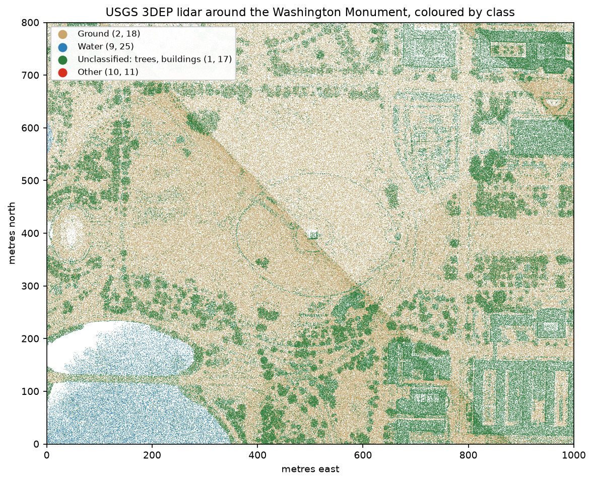
• Classes 17, 18 and 25. In the LAS 1.4 standard, 17 means “bridge deck” and 18 “high noise”. In this 2014 USGS project, however, the vendor stored points from overlapping flight lines as the standard class plus 16. So 18 is overlap ground, 17 is overlap unclassified and 25 is overlap water. Always read the project’s metadata report before trusting class codes: if you used only class 2 here you would throw away 59% of the ground points.

Step 4: remove noise with statistical outlier removal

Statistical outlier removal (SOR) flags points that are unusually far from their neighbours. For each point we find the 8 nearest neighbours in 3D with SciPy’s cKDTree, then flag points whose mean neighbour distance is more than three standard deviations above the average:

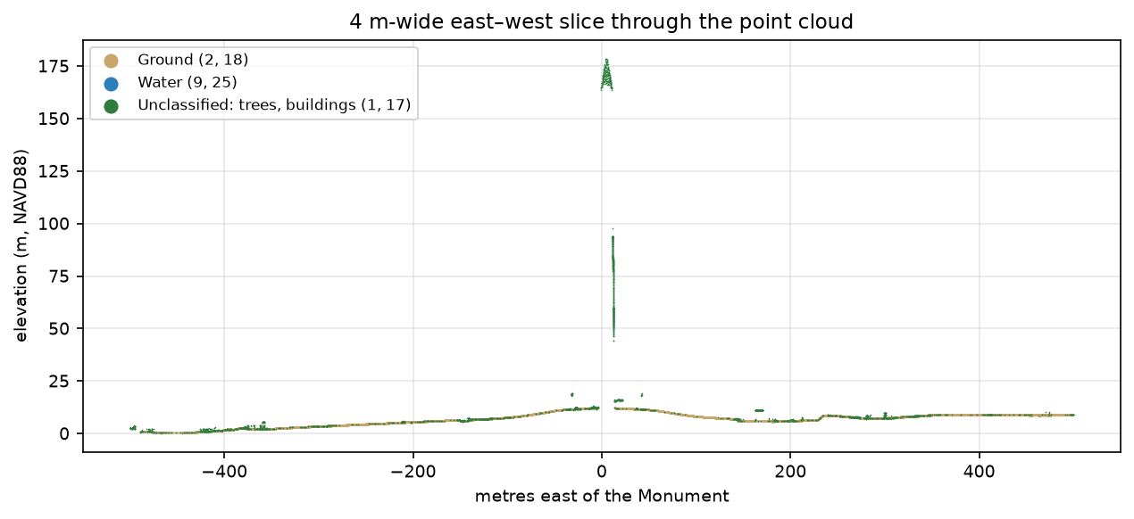
tree = cKDTree(np.c_[x, y, z])
dist, _ = tree.query(np.c_[x, y, z], k=9, workers=-1)  # nearest 8 neighbours (+ the point itself)
mean_d = dist[:, 1:].mean(axis=1)
limit = mean_d.mean() + 3 * mean_d.std()
NOISE = (cls == 7) | (mean_d > limit)
keep = ~NOISE

mean neighbour distance 0.52 m, limit 1.98 m, took 2.6 s
outliers: 11,726 (0.19%); of the 11 points above 200 m, 11 are outliers

All 11 high points are caught. The rest of the 11,726 outliers are mostly isolated returns from the edges of trees and buildings, so this costs very little detail. A side view shows what we are left with:

Step 5: grid the points into a DSM and DTM

To turn points into rasters, compute which 1 m cell each point falls into. Then use NumPy’s grouped operations: np.maximum.at for the highest point per cell, and np.bincount for sums and counts.

RES = 1.0
ncol, nrow = int((xmax - xmin) / RES), int((ymax - ymin) / RES)
col = np.clip(((x - xmin) / RES).astype(int), 0, ncol - 1)
row = np.clip(((ymax - y) / RES).astype(int), 0, nrow - 1)
cell = row * ncol + col

# DSM: highest non-noise return in each cell.
dsm = np.full(nrow * ncol, -np.inf)
np.maximum.at(dsm, cell[keep], z[keep])
dsm[np.isinf(dsm)] = np.nan
dsm = dsm.reshape(nrow, ncol)

# DTM: mean of ground and water returns (water is the "ground" of a lake) in each cell.
GROUND = np.isin(cls, [2, 18])
WATER = np.isin(cls, [9, 25])
terrain = (GROUND | WATER) & keep
gsum = np.bincount(cell[terrain], weights=z[terrain], minlength=nrow * ncol)
gcnt = np.bincount(cell[terrain], minlength=nrow * ncol)
dtm = np.where(gcnt > 0, gsum / np.maximum(gcnt, 1), np.nan).reshape(nrow, ncol)

DSM cells with no return: 1.1%
DTM cells with no ground point: 13.9%

The DTM has holes wherever buildings and dense trees hide the ground. We fill them with linear interpolation (scipy.interpolate.griddata), then fill anything left at the edges with the nearest value:

rr, cc = np.nonzero(~np.isnan(dtm))
hr, hc = np.nonzero(np.isnan(dtm))
dtm[hr, hc] = griddata((rr, cc), dtm[rr, cc], (hr, hc), method="linear")
for arr in (dtm, dsm):  # anything left (edges, outside the convex hull): nearest neighbour
    holes = np.isnan(arr)
    if holes.any():
        idx = ndimage.distance_transform_edt(holes, return_distances=False, return_indices=True)
        arr[holes] = arr[tuple(idx)][holes]
ndsm = np.clip(dsm - dtm, 0, None)

gap filling: 25.0 s
DTM -8.4..13.3 m | DSM -17.6..180.5 m | height above ground max 168.2 m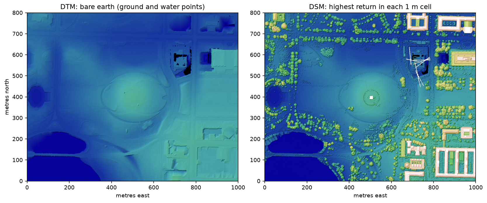

Step 6: the normalised DSM

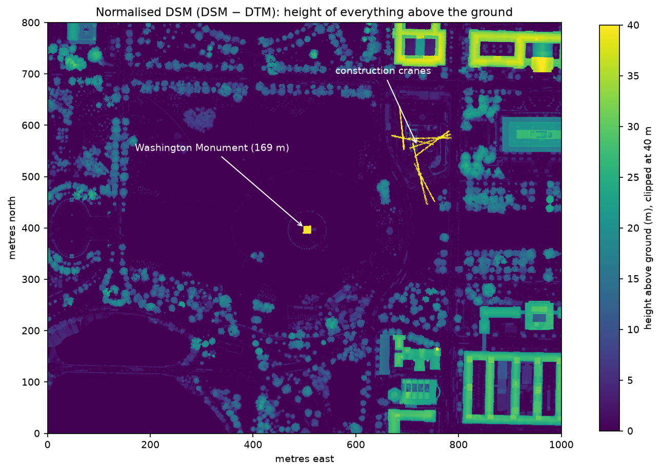
Subtracting the DTM from the DSM gives the normalised DSM (nDSM), the height of everything above the local ground, independent of the terrain:

Step 7: build a canopy height model

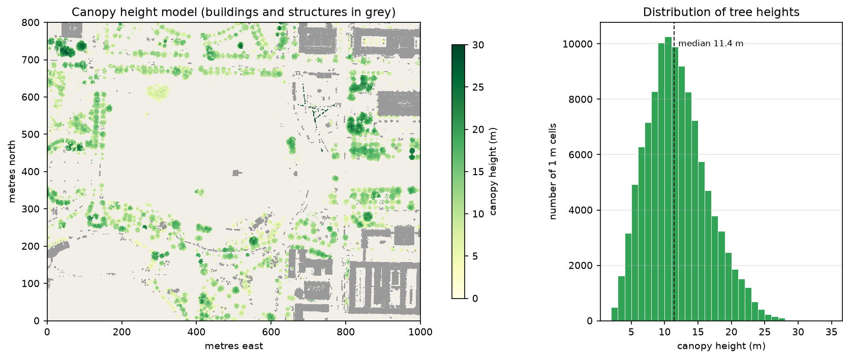
The nDSM mixes trees and buildings. A proper canopy height model needs only the trees. Many datasets, including this one, do not classify vegetation, so we use the physics instead. A laser pulse that hits a tree crown usually splits into several returns, while one that hits a roof gives a single return. In each cell more than 2 m above ground, we measure the share of points that came from multi-return pulses:

height_pt = z - dtm.ravel()[cell]
tall = keep & ~GROUND & ~WATER & (height_pt > 2)
multi = np.bincount(cell[tall & (nr > 1)], minlength=nrow * ncol)
alln = np.bincount(cell[tall], minlength=nrow * ncol)
frac = np.where(alln > 0, multi / np.maximum(alln, 1), 0).reshape(nrow, ncol)
elevated = ndsm > 2
# Laser pulses split into several returns in tree crowns but not on solid roofs.
veg = ndimage.binary_opening(elevated & (frac >= 0.5), iterations=1)
struct = ndimage.binary_opening(elevated & (frac < 0.5), iterations=1)
chm = np.where(veg, ndsm, 0.0)

The binary_opening removes single stray cells along roof edges, where a pulse can split between the roof and the ground.

cells more than 2 m above ground: 28.7%
  mostly multi-return (trees): 14.2% | mostly single-return (buildings, structures): 10.0%
tree canopy height: median 11.4 m, 95th percentile 20.5 m, max 78.7 m
canopy patches of 20 m² or more: 363
wrote output/dtm.tif, output/dsm.tif, output/chm.tif

The remaining 4.5% of elevated cells are the thin edges removed by the opening.

Finally, save the rasters as GeoTIFFs with the lidar’s CRS, so they open in QGIS or any other GIS:

transform = from_origin(xmin, ymax, RES, RES)
crs = CRS.from_wkt(header.parse_crs().to_wkt())
for name, arr in [("dtm", dtm), ("dsm", dsm), ("chm", chm)]:
    with rasterio.open(OUT / f"{name}.tif", "w", driver="GTiff", height=nrow, width=ncol, count=1,
                       dtype="float32", crs=crs, transform=transform, compress="deflate", nodata=-9999) as dst:
        dst.write(arr.astype("float32"), 1)

Step 8: check the result against the Washington Monument

How good is it? We take the highest point within 10 m of the Monument’s centre and subtract the median ground height in a ring 15–30 m away:

d = np.hypot(x - mx, y - my)
near = (d < 10) & keep
top_i = np.argmax(np.where(near, z, -np.inf))
ring = GROUND & keep & (d > 15) & (d < 30)
base = np.median(z[ring])
height = z[top_i] - base

highest point within 10 m: z=180.52 m at 5.7 m from the centre (class 17, return 1 of 1)
ground 15–30 m from the centre: median z=11.91 m from 15,280 ground points
lidar height: 168.61 m (553.2 ft)
official height (NGS survey): 169.046 m; difference -0.44 m

The lidar height is 168.61 m against the surveyed 169.046 m, 44 cm short. That is a good result: with 7.7 points per m², the chance of a pulse hitting the exact 1 m² aluminium tip is small, so lidar tends to slightly underestimate the height of spires and poles. The highest return is 5.7 m from the centre, on the pyramidion’s sloping face.

Frequently asked questions

What is the difference between a DTM, a DSM and a CHM?

A DSM (digital surface model) is the top surface: roofs, tree crowns and the ground where nothing covers it. A DTM (digital terrain model) is the bare earth with everything above it removed. A CHM (canopy height model) is the height of vegetation above the ground, DSM − DTM in tree cells. “DEM” is a general term that usually means a DTM.

How do I read a LAZ file in Python?

Install laspy with a LAZ backend (pip install "laspy[lazrs]"), then call las = laspy.read("file.laz"). Coordinates are in las.x, las.y and las.z, and attributes such as las.classification and las.intensity are NumPy-compatible arrays. For large files, use laspy.open() with chunk_iterator().

Should I use laspy or PDAL?

laspy is a pure Python reader and writer: easy to install with pip, and ideal when you want points as NumPy arrays and full control. PDAL is a C++ processing engine with ready-made filters for ground classification (SMRF, CSF), reprojection and rasterising, driven by JSON pipelines. Use PDAL for heavy production pipelines, and laspy for analysis, learning and custom algorithms. They read the same files.

Where can I download free lidar data?

The USGS 3DEP programme covers most of the United States, and it is on the Planetary Computer and AWS as COPC. OpenTopography hosts lidar from around the world. Many national mapping agencies publish their own lidar, including the Environment Agency in England, Denmark, the Netherlands (AHN) and New Zealand (LINZ). See our data sources directory.

What resolution should a DTM from lidar be?

Pick a cell size where most cells contain at least one ground point. Here about 57% of the 7.7 points per m² are ground (classes 2 and 18), roughly 4.4 ground points per m², so 1 m cells work well and only 13.9% need interpolating, mostly under buildings. Sparser or densely forested data may need 2 m or more.

Next steps

• Turn the DSM into a 3D-printable city model with From DEM to 3D-printable STL with Python.
• Compute slope, aspect and hillshade from the DTM with Terrain analysis in Python with rasterio and rioxarray.
• Vectorise building footprints from the struct mask with rasterio.features.shapes and give each one a height from the nDSM.
• Swap the multi-return rule for PDAL’s SMRF ground filter on an unclassified point cloud.
• Pair lidar with radar: Sentinel-1 SAR flood mapping in Python uses the same STAC and Planetary Computer pattern.

Data and licences

• USGS 3DEP lidar, project MD_VA_Sandy_NCR_2014 (collected 2014, tiles 18SUJ322305 and 18SUJ322306): U.S. Geological Survey, public domain. Accessed as COPC from the Microsoft Planetary Computer on 15 October 2026.
• Official Monument height: NOAA National Geodetic Survey, 2013–14 survey (554 ft 7 11/32 in, 169.046 m).
• Code: lidar_dtm_chm.py, tested with Python 3.12.0, laspy 2.7.0, lazrs 0.8.2, numpy 2.5.4, scipy 1.18.1 and rasterio 1.5.2.