InSAR ground subsidence in Python: one year of Mexico City sinking, from Sentinel-1

Short answer: to map ground subsidence with InSAR in Python, take Sentinel-1 interferograms that are already unwrapped, for example from COMET LiCSAR or ASF HyP3. Convert the unwrapped phase to line-of-sight displacement with d = −λ/(4π) · φ, which is 4.41 mm per radian for Sentinel-1. Mask pixels with low coherence and subtract a stable reference point. For one pair, that is your displacement map. For a time series, stack many short pairs and solve for the displacement at each date by least squares (SBAS). Fit a line to get a velocity, and divide by the up component of the line of sight to get vertical subsidence.

Mexico City is one of the fastest-sinking cities in the world. It is built on the soft clay of a drained lake. As groundwater is pumped from the aquifer beneath, the clay compacts and the ground drops, in places by tens of centimetres a year. That cracks buildings, tilts the cathedral, breaks pipes and changes the slope of the drains. It is also a perfect InSAR target: the city is large, dry for half the year and full of buildings that reflect radar consistently.

In this tutorial we measure one year of that motion, from September 2025 to September 2026, using real Sentinel-1 interferograms. You will learn how to:

1. find and stream pre-processed interferograms from the free COMET LiCSAR archive, reading only the window you need;
2. understand wrapped and unwrapped phase, line of sight and coherence on a single interferogram;
3. build a coherence mask and choose a reference point;
4. invert a network of 170 interferograms into a displacement time series (SBAS) with one NumPy least-squares call;
5. produce a velocity map, a profile and time series, and a GeoTIFF;
6. cross-check the result with MintPy, the standard open-source InSAR time-series package.

All outputs below are real results from insar_subsidence.py and mintpy_crosscheck.py, run in October 2026 with Python 3.12, rasterio 1.5.2, NumPy 2.5.4 and MintPy 1.6.4. If you are new to radar, read Sentinel-1 SAR flood mapping in Python first; it explains backscatter, polarisation and speckle.

How InSAR measures millimetres from 700 km away

Sentinel-1 is a C-band radar with a wavelength (λ) of 5.55 cm. Every pixel of a complex radar image (a SLC, single look complex) has an amplitude, which is the brightness used in flood mapping, and a phase: where in its 5.55 cm cycle the wave was when the echo returned. The phase of a single image is random, because each pixel contains many scatterers. But if the satellite images the same place again from almost the same position, and nothing in the pixel has changed, that random part cancels when you subtract the two phases.

What remains is the change in the two-way distance between the satellite and the ground. If the ground moves 1 cm away from the satellite, the echo travels 2 cm further, so the phase changes by 4π × 0.01 / λ. An interferogram is an image of this phase difference, after removing the known effects of orbit geometry and topography.

Three ideas matter for everything that follows:

• Wrapped phase. Phase is only known modulo 2π: it runs from −π to π and then starts again. Each full cycle of colour, called a fringe, is half a wavelength of line-of-sight motion: 27.7 mm for Sentinel-1.
• Unwrapped phase. Unwrapping adds the right number of 2π cycles to each pixel to make the phase continuous. It is the hardest step in InSAR processing. Errors appear as jumps of exactly 2π (27.7 mm).
• Line of sight (LOS). The radar only measures motion towards or away from the satellite, along a line tilted 30–46° from vertical. A pixel that sinks moves away from the satellite. A pixel that moves sideways can also change its distance to the satellite.

Step 1: list the LiCSAR interferograms for Mexico City

LiCSAR organises its products by Sentinel-1 frame. Frame 143D_07132_131313 is on relative orbit 143, descending (the satellite flies south and looks west), and covers the Valley of Mexico. Each interferogram is a folder named <first date>_<second date> that holds geocoded GeoTIFFs: .geo.unw.tif (unwrapped phase, radians), .geo.cc.tif (coherence, scaled 0–255) and .geo.diff_pha.tif (wrapped phase).

We list the folder and keep only short pairs of up to 18 days. Short pairs keep coherence high, because the ground surface has little time to change.

FRAME = "143D_07132_131313"     # Sentinel-1 relative orbit 143, descending
BASE = f"https://gws-access.jasmin.ac.uk/public/nceo_geohazards/LiCSAR_products.public/143/{FRAME}"
BBOX = (-99.30, 19.20, -98.80, 19.60)  # lon/lat window: Mexico City, Nezahualcoyotl and Chalco
START, END = "20250911", "20260913"     # one year of 6-day Sentinel-1 acquisitions
MAX_DAYS = 18                           # keep only short temporal baselines: 6, 12 and 18 days
WAVELENGTH = 0.0554658                  # Sentinel-1 C-band wavelength in metres
RAD2MM = -WAVELENGTH / (4 * np.pi) * 1000  # LiCSAR convention: positive = towards the satellite


def days(pair: str) -> int:
    return (datetime.strptime(pair[9:], "%Y%m%d") - datetime.strptime(pair[:8], "%Y%m%d")).days


html = requests.get(f"{BASE}/interferograms/", timeout=60).text
all_pairs = sorted(set(re.findall(r'href="(\d{8}_\d{8})/"', html)))
pairs = [p for p in all_pairs if p[:8] >= START and p[9:] <= END and days(p) <= MAX_DAYS]
epochs = sorted({p[:8] for p in pairs} | {p[9:] for p in pairs})
meta = dict(line.split("=", 1) for line in requests.get(f"{BASE}/metadata/metadata.txt", timeout=60).text.split()
            if "=" in line)

frame 143D_07132_131313: 4,434 interferograms online, 20141003 to 20260913
selected: 170 pairs of <= 18 days between 61 epochs, 20250911 to 20260913
temporal baselines (days): {5: 1, 6: 54, 7: 2, 12: 56, 13: 2, 18: 55}
heading -169.2°, mean incidence 33.9°

The frame has been imaged every 6 or 12 days since October 2014. Our year has 61 acquisitions joined by 170 interferograms. Each date is linked to the next three dates where they exist, which gives 6-, 12- and 18-day pairs. A few acquisitions were shifted by a day, hence the odd 5-, 7- and 13-day pairs.

Step 2: stream only the window you need

A LiCSAR frame is hundreds of kilometres across. We need a 53 × 44 km window around the city. The GeoTIFFs are compressed in strips of one row, so rasterio can read just the rows that cover our window over HTTP. That is much faster than downloading 340 whole files. We cache the stack locally after the first run.

def read_window(url: str):
    """Read only the rows of a remote LiCSAR GeoTIFF that cover BBOX (HTTP range requests)."""
    with rasterio.open(url) as src:
        win = from_bounds(*BBOX, src.transform).round_offsets().round_lengths()
        return src.read(1, window=win), src.window_transform(win)


unw, coh = [], []
for p in pairs:
    u, transform = read_window(f"{BASE}/interferograms/{p}/{p}.geo.unw.tif")
    c, _ = read_window(f"{BASE}/interferograms/{p}/{p}.geo.cc.tif")
    unw.append(u)
    coh.append(c)
unw, coh = np.array(unw, "float32"), np.array(coh, "uint8")
coh = coh.astype("float32") / 255                      # LiCSAR stores coherence as 0-255
unw[unw == 0] = np.nan                                 # 0 = not unwrapped (masked by LiCSAR)
up = read_window(f"{BASE}/metadata/{FRAME}.geo.U.tif")[0]   # up component of the LOS unit vector
hgt = read_window(f"{BASE}/metadata/{FRAME}.geo.hgt.tif")[0].astype("float32")

170 interferograms x 400 x 500 pixels (3.6 arcsec, about 105 m x 111 m)
unwrapped in every pair: 94.3% of pixels; LOS up component 0.695..0.733 (local incidence 44.5°)

LiCSAR also publishes the line-of-sight unit vector for every pixel (.geo.E/N/U.tif) and the DEM it used (.geo.hgt.tif). The up component, about 0.71, tells us that Mexico City is near the far edge of the swath, where the radar looks 44.5° from vertical. The frame average is 33.9°.

Step 3: wrapped phase, unwrapped phase and coherence

Before building a time series, look at a single interferogram. We picked a 60-day pair from the dry season, 3 January to 4 March 2026, because its fringes are clear.

REF = (-99.185, 19.325)                 # stable reference: Pedregal lava field, Ciudad Universitaria
SHOWCASE = "20260103_20260304"          # a 60-day dry-season pair to show wrapped vs unwrapped phase

inv = ~transform
rc, rr = (int(v) for v in inv * REF)
ref_win = (slice(rr - 2, rr + 3), slice(rc - 2, rc + 3))   # 5 x 5 pixel reference area
wrapped, _ = read_window(f"{BASE}/interferograms/{SHOWCASE}/{SHOWCASE}.geo.diff_pha.tif")
show_unw, _ = read_window(f"{BASE}/interferograms/{SHOWCASE}/{SHOWCASE}.geo.unw.tif")
show_coh, _ = read_window(f"{BASE}/interferograms/{SHOWCASE}/{SHOWCASE}.geo.cc.tif")
show_unw[show_unw == 0] = np.nan
show_coh = show_coh / 255
show_los = (show_unw - np.nanmedian(show_unw[ref_win])) * RAD2MM

wrapped phase range -3.14..3.14 rad; unwrapped 1.2..16.8 rad
one fringe (2π) = 27.7 mm of LOS motion
LOS change relative to CU: 1st percentile -33 mm, 99th percentile 16 mm
median coherence 0.52; pixels with coherence < 0.3: 25.2%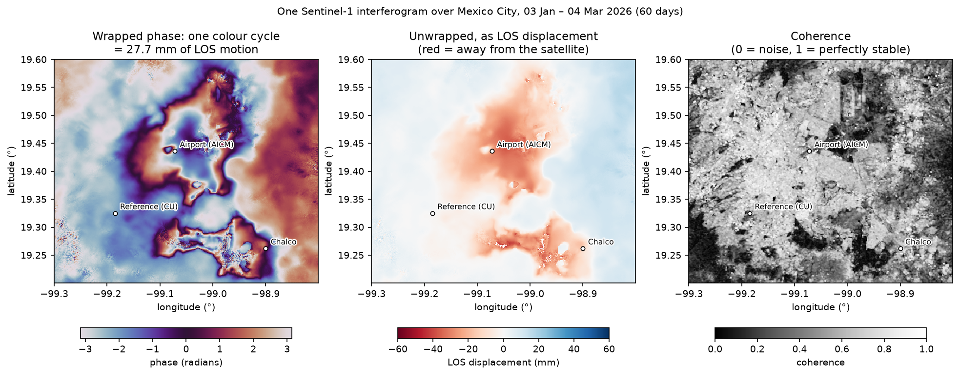

The wrapped phase on the left shows two bowls of fringes: one around the airport and Nezahualcóyotl, and one around Tláhuac and Chalco in the south-east. Counting the fringes gives the motion: one or two cycles, so 30–55 mm in 60 days. Unwrapping (middle) replaces the repeating colours with one continuous number. Relative to the reference at CU, the ground in the centre of the bowls moved up to about 33 mm away from the satellite in two months (the 1st percentile).

The coherence map on the right explains where the measurements are trustworthy. Buildings and roads keep the same scatterers for months and stay bright. Vegetated hills, fields and the seasonally wet remnants of Lake Texcoco north-east of the airport change between visits and are dark.

Step 4: coherence mask and reference point

A single 60-day pair is noisy. We now use all 170 short pairs. First, average their coherence and keep pixels with a mean coherence of at least 0.35 that were unwrapped in every pair. Then pick a reference point: InSAR measures only relative motion, so every interferogram is shifted so that a stable area has zero displacement.

We chose the Pedregal de San Ángel lava field under Ciudad Universitaria (CU), in the south-west of the city. It is solid basalt, not clay, so it should not subside. Using the median of a 5 × 5 pixel window, rather than one pixel, makes the reference less sensitive to noise.

mean_coh = coh.mean(0)
mask = (mean_coh >= 0.35) & np.isfinite(unw).all(0)
mask = ndimage.binary_opening(mask, iterations=1)
unw_ref = unw - np.nanmedian(unw[:, ref_win[0], ref_win[1]].reshape(n_ifg, -1), axis=1)[:, None, None]

mean coherence: median 0.59; reference area 0.61
kept 150,831 of 200,000 pixels (75.4%) with mean coherence >= 0.35 and unwrapped in all 170 pairs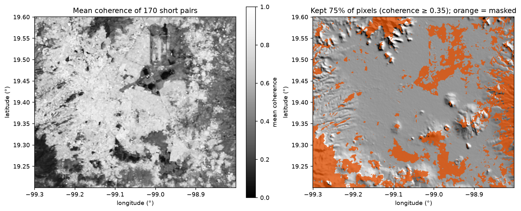

The city itself is almost entirely kept. The masked holes are the forested Sierra de las Cruces in the south-west, the fields of the south-east, and the wetland remnants of Lake Texcoco and Lake Chalco. The threshold of 0.35 is a judgement call. A higher threshold gives cleaner but sparser results.

Step 5: invert the network into a time series (SBAS)

Each interferogram measures the displacement between two dates. We want the displacement at each date. With 61 dates, there are 60 unknowns (the first date is zero by definition) and 170 observations. That is an over-determined linear system, A · x = φ, where each row of the design matrix A has −1 at the first date of a pair and +1 at the second.

This is the small baseline subset (SBAS) method. It is the core of MintPy, LiCSBAS and most InSAR time-series software. Because every pixel shares the same A, NumPy can solve all 150,831 pixels in one call.

dates = pd.to_datetime(epochs)
t_years = np.array((dates - dates[0]).days) / 365.25
idx = {e: i for i, e in enumerate(epochs)}
A = np.zeros((n_ifg, len(epochs) - 1))     # unknowns: phase at each epoch after the first
for k, p in enumerate(pairs):
    i, j = idx[p[:8]], idx[p[9:]]
    A[k, j - 1] = 1
    if i > 0:
        A[k, i - 1] = -1
obs = unw_ref[:, mask]                         # n_ifg x n_pixels
x, *_ = np.linalg.lstsq(A, obs, rcond=None)
resid = obs - A @ x
ts = np.full((len(epochs), H, W), np.nan, "float32")
ts[0, mask] = 0
ts[1:, mask] = x * RAD2MM                      # cumulative LOS displacement in mm
rms_ifg = np.sqrt(np.mean(resid ** 2, axis=1)) * abs(RAD2MM)

design matrix (170, 60), rank 60 (needs 60: one connected network)
residual RMS per interferogram: median 0.15 mm, max 0.39 mm (20251011_20251029)
pixels with a residual > π in any pair (likely unwrapping errors): 0.01%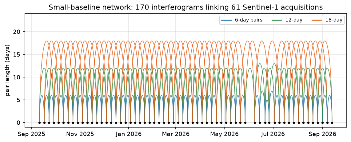

Two checks matter here:

• Rank. If the network splits into disconnected groups, A is rank-deficient and the time series of each group floats freely. Rank 60 confirms one connected network. MintPy and LiCSBAS warn about this too.
• Residuals. Because there are more interferograms than dates, the inversion cannot fit inconsistent pairs exactly. An unwrapping error in one interferogram shows up as a residual of about 2π. Only 0.01% of pixels have a residual larger than π, so the LiCSAR unwrapping is very consistent here. The largest per-pair RMS is 0.39 mm.

Step 6: velocity, vertical subsidence and a GeoTIFF

Fitting a straight line through each pixel’s time series gives the mean LOS velocity. To turn LOS into vertical motion, divide by the up component of the line-of-sight vector. That assumes the ground only moves vertically, which is a reasonable assumption for subsidence on the flat lakebed. We also estimate a simple 1σ uncertainty from the scatter of each time series around its line.

G = np.column_stack([np.ones_like(t_years), t_years])
coef, *_ = np.linalg.lstsq(G, ts[:, mask], rcond=None)
v_los = np.full((H, W), np.nan, "float32")
v_los[mask] = coef[1]
fit_resid = ts[:, mask] - G @ coef
v_std = np.full((H, W), np.nan, "float32")
v_std[mask] = np.sqrt((fit_resid ** 2).sum(0) / (len(epochs) - 2) / ((t_years - t_years.mean()) ** 2).sum())
v_up = v_los / up                             # assumes the motion is purely vertical

with rasterio.open(OUT / "vertical_velocity_mm_yr.tif", "w", driver="GTiff", height=H, width=W, count=1,
                   dtype="float32", crs="EPSG:4326", transform=transform, nodata=np.nan, compress="deflate") as dst:
    dst.write(v_up, 1)

LOS velocity: 1st percentile -215 mm/yr, median -8 mm/yr, 99th percentile 9 mm/yr
vertical (LOS / up component): fastest -383 mm/yr; area subsiding faster than 100 mm/yr: 367 km², faster than 200 mm/yr: 136 km²
median 1-sigma velocity uncertainty (scatter about the line): 3.4 mm/yr
           place  height_m  coherence  los_mm_yr  vertical_mm_yr  los_total_mm
          Chalco      2242       0.70     -113.9          -156.9         -96.0
         Tláhuac      2238       0.72     -156.6          -218.0        -145.4
  Nezahualcóyotl      2236       0.74     -199.7          -278.7        -195.4
  Airport (AICM)      2226       0.35     -170.1          -238.8        -176.1
Centro Histórico      2242       0.72      -87.5          -123.7         -89.2
  Reference (CU)      2290       0.65        0.1             0.1           0.2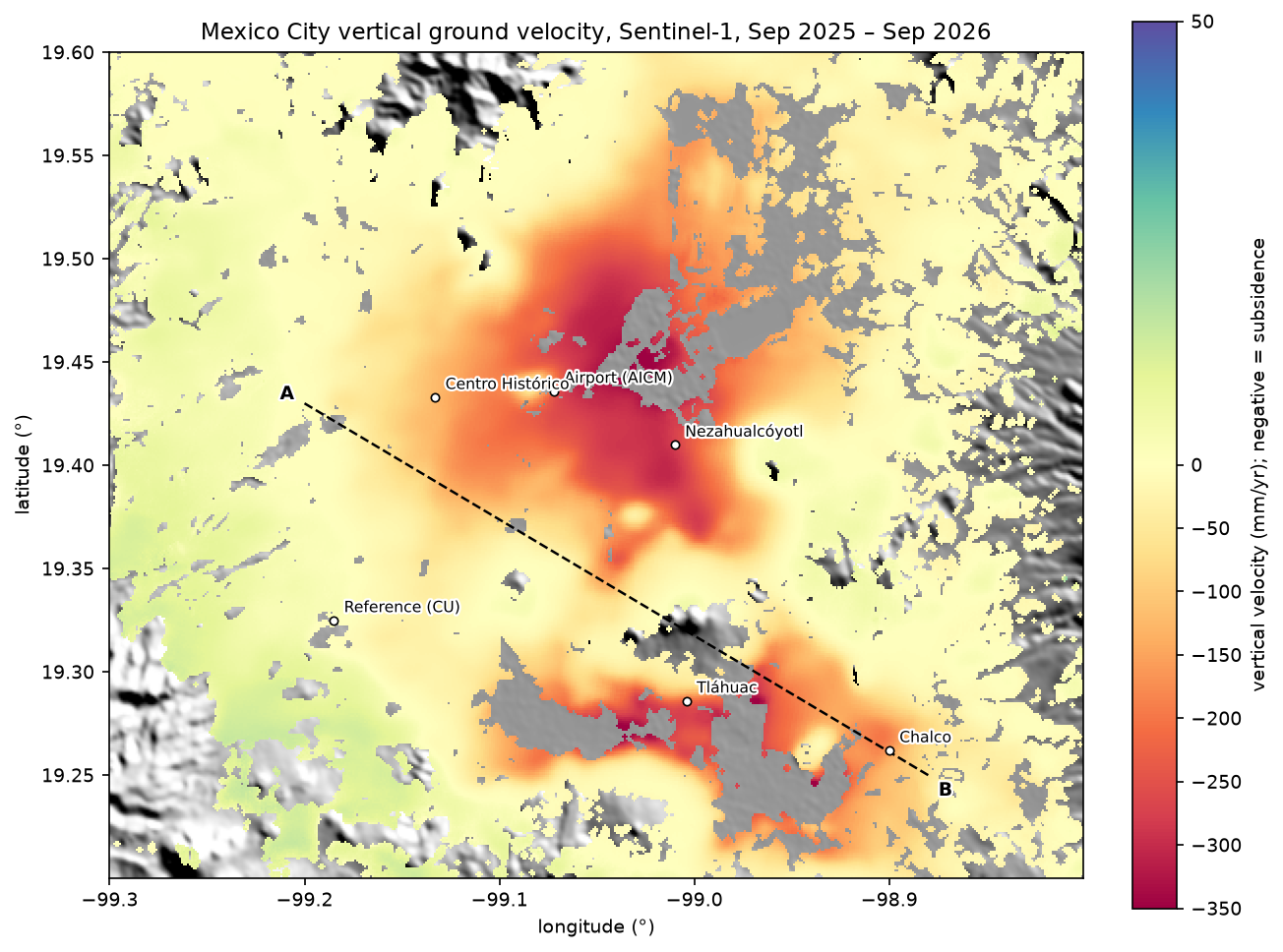

The map shows the classic Mexico City pattern. The western and southern parts of the city stand on volcanic rock and alluvial fans and are almost stable. The subsidence bowls follow the old lakebed: the north-east around the airport and Nezahualcóyotl, and the former Lake Xochimilco–Chalco basin in the south-east. In one year, 367 km² sank faster than 10 cm a year, and 136 km² sank faster than 20 cm a year. These rates are in the same range as published Sentinel-1 studies of the city, which report up to about 40 cm a year in the fastest areas.

The airport point has a mean coherence of exactly 0.35, on the edge of the mask, so treat its value with more caution than the others.

Step 7: a profile across the basin

A profile makes the link between geology and subsidence clear. We sample the velocity and the DEM along a 39 km line from Chapultepec Park in the west to Chalco in the south-east.

PROFILE = ((-99.20, 19.43), (-98.88, 19.25))  # Chapultepec to Chalco, through the old lakebed
(lon0, lat0), (lon1, lat1) = PROFILE
n = 400
plon, plat = np.linspace(lon0, lon1, n), np.linspace(lat0, lat1, n)
pc, pr = inv * (plon, plat)
dist_km = np.hypot((plon - lon0) * 111.32 * np.cos(np.radians(19.4)), (plat - lat0) * 110.6)
prof_v = ndimage.map_coordinates(np.where(mask, v_up, -9999), [pr - 0.5, pc - 0.5], order=0, cval=-9999)
prof_v = np.where(prof_v < -9000, np.nan, prof_v)
prof_h = ndimage.map_coordinates(hgt, [pr - 0.5, pc - 0.5], order=1)

length 39.1 km; valid samples 81%; fastest -260 mm/yr at 28.6 km; terrain 2234-2563 m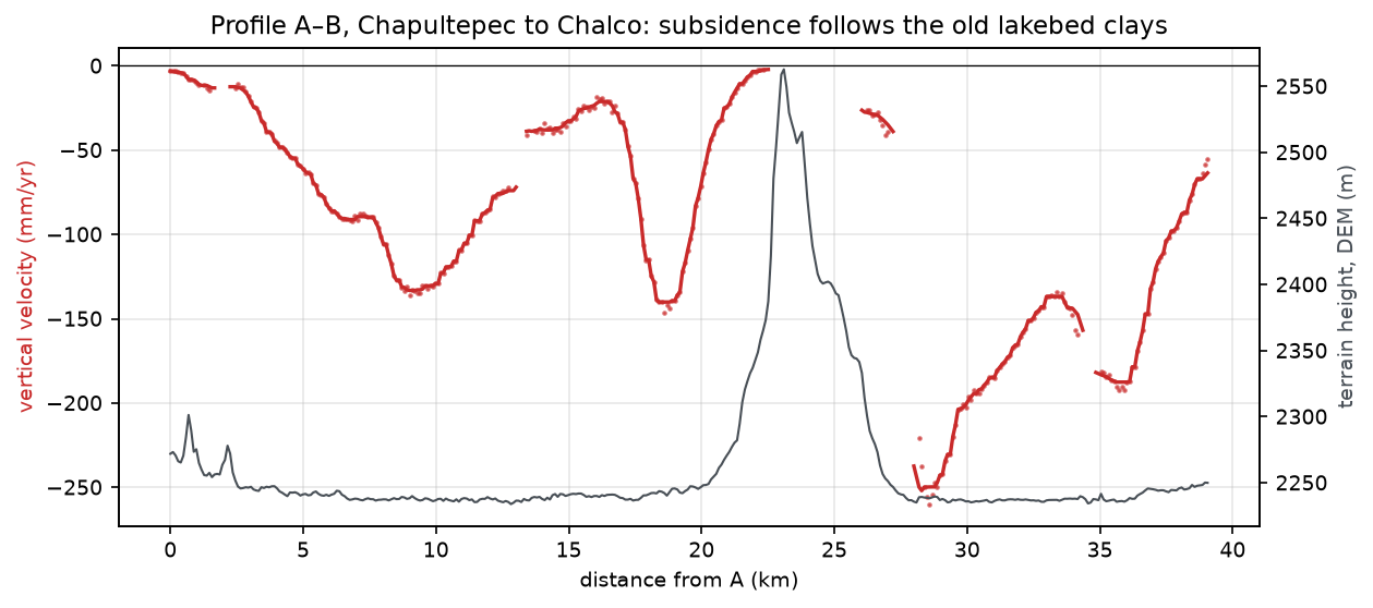

The profile is flat at about 2,240 m for most of its length: this is the old lake floor. The one exception is the Sierra de Santa Catarina, a chain of young volcanoes that rises to 2,560 m at 23 km. Its velocity is close to zero. A few kilometres either side, on clay, the ground sinks by 140 to 260 mm a year. The rate depends on the thickness of the compressible clay, not on the terrain height, which is why subsidence changes so sharply at the edges of the old lake.

Step 8: time series at points

The velocity is an average. The time series shows how steady the motion is and how noisy the individual dates are.

POINTS = {"Chalco": (-98.900, 19.262), "Tláhuac": (-99.004, 19.286),
          "Nezahualcóyotl": (-99.010, 19.410),
          "Airport (AICM)": (-99.072, 19.436), "Centro Histórico": (-99.133, 19.433),
          "Reference (CU)": REF}


def window_median(arr: np.ndarray, lon: float, lat: float, half: int = 1):
    c, r = (int(v) for v in inv * (lon, lat))
    return np.nanmedian(arr[..., r - half:r + half + 1, c - half:c + half + 1].reshape(*arr.shape[:-2], -1), -1)


series = pd.DataFrame({name: window_median(ts, *xy) for name, xy in POINTS.items()}, index=dates)
series.round(1).to_csv(OUT / "los_timeseries_points.csv", index_label="date")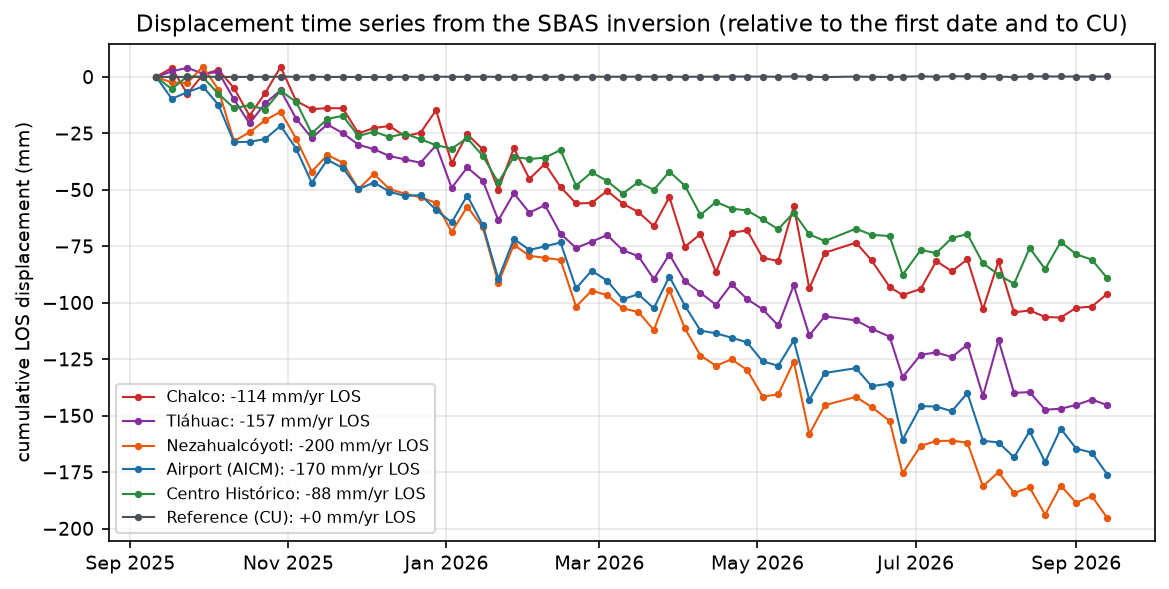

Subsidence in Mexico City is remarkably steady: the lines fall almost straight. In one year, Nezahualcóyotl moved 195 mm away from the satellite, which is about 28 cm of vertical subsidence a year. Notice that all the curves zigzag together. When one date is too high, it is too high everywhere. That is the signature of the atmosphere: water vapour slows the radar wave, and a change in humidity between two dates looks like a change in distance. It is strongest in the summer rainy season.

Step 9: cross-check with MintPy

MintPy (the Miami INsar Time-series software in PYthon) is the most widely used open-source InSAR time-series package. It reads stacks from ISCE, HyP3, LiCSAR, GAMMA and SNAP, and adds weighting, unwrapping-error correction, tropospheric correction (for example with ERA5 or GACOS), DEM-error correction and much more.

Our main script also writes the referenced stack in MintPy’s own HDF5 layout (ifgramStack.h5). That lets MintPy invert exactly the same data, so we can check our NumPy version. With --weight-func no, MintPy uses unweighted least squares, the same estimator as np.linalg.lstsq.

import contextlib
import os
from pathlib import Path

import h5py
import mintpy
import numpy as np
from mintpy.cli import ifgram_inversion, timeseries2velocity

HERE = Path(__file__).parent
DATA = HERE / "data"
os.chdir(DATA)
print(f"MintPy {mintpy.__version__}")

# Unweighted least squares: the same estimator as np.linalg.lstsq. MintPy's progress log goes to mintpy.log.
with open("mintpy.log", "w") as log, contextlib.redirect_stdout(log):
    ifgram_inversion.main(["ifgramStack.h5", "--weight-func", "no", "--update"])
    timeseries2velocity.main(["timeseries.h5", "-o", "velocity.h5", "--update"])

with h5py.File("timeseries.h5") as f:
    ts = f["timeseries"][:]                    # metres, positive = towards the satellite
    dates = [d.decode() for d in f["date"][:]]
with h5py.File("velocity.h5") as f:
    v_mintpy = f["velocity"][:] * 1000         # m/yr -> mm/yr
mask = np.load("mask.npy")
v_numpy = np.load("v_los_numpy.npy")
diff = v_mintpy[mask] - v_numpy[mask]

MintPy 1.6.4

MintPy time series: 61 dates, 20250911 to 20260913
LOS velocity, MintPy: 1st percentile -214 mm/yr, median -7 mm/yr
MintPy minus NumPy over 150,831 pixels: mean +0.62 mm/yr, max |difference| 0.83 mm/yr, correlation 1.0000

The two results agree to within 0.83 mm a year everywhere, with a correlation of 1.0000. The small constant offset of +0.62 mm a year comes from the reference: MintPy references to a single pixel, while we used the median of a 5 × 5 window.

For a full MintPy workflow, you would point smallbaselineApp.py at a config file instead. It loads the LiCSAR or HyP3 GeoTIFFs, and then runs the same network inversion, plus corrections, in about a dozen steps. Understanding the inversion in NumPy first makes MintPy’s outputs much easier to interpret and debug.

Limitations and caveats

• Line of sight only. One track measures one component of motion. Converting to vertical assumes no horizontal motion. That is reasonable in the middle of the basin but not at its edges, where the ground also moves sideways towards the centre of the bowl. Combining this descending track with an ascending one (LiCSAR frames 078A_07049_131313 or 005A_07021_131313 cover the city) lets you solve for vertical and east–west motion separately.
• Everything is relative. The velocities are relative to CU. If the reference itself moves, every value shifts by the same amount. Choose a reference on rock, check it in several interferograms, and consider GNSS stations (Mexico City has several) to tie the result to an absolute frame.
• Atmosphere. Tropospheric delay changes from day to day, especially in the rainy season, and is also correlated with height. Over a year, it averages down for a steady signal like this one, but our simple uncertainty of 3.4 mm a year treats the noise as random and so is optimistic. MintPy can apply ERA5 or GACOS corrections. LiCSAR also publishes GACOS correction files for many frames.
• Unwrapping errors. Errors in multiples of 27.7 mm can occur where coherence is low or the motion is fast between dates. Short pairs help, and the residual check flags inconsistent pixels.
• Coherence holes. The wettest parts of the ex-lakes, which are among the fastest-sinking areas, are masked because the surface changes too much. Persistent scatterer methods, or a lower threshold with more care, can recover some of them.
• Fast motion and resolution. At about 100 m pixels, LiCSAR products average over whole blocks. For individual buildings or metro lines, process full-resolution SLC data with tools such as ISCE2, SNAP and StaMPS, or with MintPy’s or MiaplPy’s own workflows.
• Data source. We used LiCSAR because it needs no login. ASF HyP3 offers the same kind of product on demand anywhere in the world, with a free NASA Earthdata account, and MintPy reads it directly.

Frequently asked questions

What is InSAR and how does it measure subsidence?

InSAR compares the phase of two radar images of the same place taken at different times. A change in phase means a change in the distance between the ground and the satellite. Sentinel-1 radar has a wavelength of 5.55 cm, so a full phase cycle corresponds to 27.7 mm of line-of-sight motion, and careful processing can detect motion of a few millimetres. Subsidence shows up as ground moving away from the satellite.

Is Sentinel-1 InSAR data free?

Yes. Sentinel-1 images are free under the Copernicus licence. Pre-processed interferograms are also free: COMET LiCSAR publishes them openly for many areas, and ASF HyP3 makes them on demand with a free NASA Earthdata login. The European Ground Motion Service (EGMS) also publishes ready-made velocity maps for most of Europe.

What is the difference between wrapped and unwrapped phase?

Wrapped phase is the raw phase difference, known only between −π and π, so it repeats in fringes. Unwrapped phase adds the right number of whole cycles to each pixel to make a continuous surface, which you can convert directly to millimetres. Unwrapping is done during processing, for example with SNAPHU in LiCSAR, and errors appear as jumps of exactly one fringe.

Why do I need many interferograms instead of one?

A single interferogram measures the motion between two dates, but it also contains atmospheric delay, which can be as large as several centimetres. Combining many short interferograms in a time series (SBAS) gives the displacement at each date, averages down the atmospheric noise and allows unwrapping errors to be detected. It also keeps coherence high, because each pair is short.

How accurate is InSAR for ground subsidence?

For a steady signal over a year or more of Sentinel-1 data, velocities are typically precise to a few millimetres a year, relative to the reference point. Single dates are noisier, at a level of about 5–10 mm, mainly because of the atmosphere. Accuracy also depends on coherence, the reference point and whether horizontal motion is present. Validating against GNSS or levelling is good practice.

What is MintPy?

MintPy is a free, open-source Python package for InSAR time-series analysis, originally developed at the University of Miami. It reads interferograms from most processors, inverts them into a time series with the small-baseline method, and applies corrections for unwrapping errors, the troposphere and DEM errors. This tutorial uses its ifgram_inversion and timeseries2velocity steps to check our NumPy inversion.

Next steps

• Add an ascending LiCSAR frame and decompose the motion into vertical and east–west components.
• Run MintPy’s smallbaselineApp.py with ERA5 or GACOS tropospheric correction and compare the time series.
• Extend the stack back to 2014 to see whether the subsidence rate has changed.
• Detect ships in the same Sentinel-1 data, using backscatter instead of phase, in Sentinel-1 ship detection in Python with CFAR.
• Use backscatter to map water in Sentinel-1 SAR flood mapping in Python.
• Combine the velocity GeoTIFF with slope and hillshade from Terrain analysis in Python with rasterio, or put it on an interactive map with Folium.

Data and licences

• COMET LiCSAR products: contain modified Copernicus Sentinel data 2025–2026, processed by COMET (LiCSAR). Open data under CC BY 4.0. Frame 143D_07132_131313, accessed from the COMET LiCSAR archive in October 2026.
• References: Lazecký, M. et al. (2020), “LiCSAR: an automatic InSAR tool for measuring and monitoring tectonic and volcanic activity”, Remote Sensing 12(15), 2430; Yunjun, Z., Fattahi, H. and Amelung, F. (2019), “Small baseline InSAR time series analysis: unwrapping error correction and noise reduction”, Computers & Geosciences 133, 104331; Berardino, P. et al. (2002), “A new algorithm for surface deformation monitoring based on small baseline differential SAR interferograms”, IEEE Transactions on Geoscience and Remote Sensing 40(11).
• Code: insar_subsidence.py and mintpy_crosscheck.py, tested with Python 3.12.0, requests 2.34.2, rasterio 1.5.2, NumPy 2.5.4, SciPy 1.18.1, h5py 3.16.0 and MintPy 1.6.4.