Sentinel-1 ship detection in Python: a CA-CFAR detector off the Port of Rotterdam

Short answer: to detect ships in Sentinel-1 SAR imagery with Python, load the VV and VH backscatter as linear power, mask the land, and run a CFAR (constant false alarm rate) detector. For each pixel, estimate the mean sea brightness in a ring around it, ignoring a guard window that holds the ship itself. Flag the pixel if it is brighter than k × mean, where k comes from a speckle model and your chosen false-alarm rate. Then group neighbouring detections into targets with scipy.ndimage.label, drop tiny ones, and remove fixed structures, sidelobes and ghosts before you count ships.

Ships are among the easiest things to find in radar images. A steel hull and superstructure form corners that reflect the radar pulse straight back, so a ship looks like a bright point on the dark sea. Radar works at night and through cloud, which is why coastguards, fisheries agencies and analysts of sanctions and dark shipping use Sentinel-1 every day.

In this tutorial we detect ships off the Port of Rotterdam, Europe’s busiest port, where the anchorages, the Maasgeul approach channel and the Hollandse Kust Zuid offshore wind farm share 2,000 km² of the North Sea. You will learn how to:

1. find Sentinel-1 RTC scenes for one orbit on the Microsoft Planetary Computer and stream them onto a 10 m grid;
2. build a land mask from ESA WorldCover;
3. write a CA-CFAR detector with scipy.ndimage.uniform_filter and set its threshold from a gamma speckle model;
4. cluster detected pixels into targets and measure them;
5. recognise the classic false alarms: wind turbines and platforms, sidelobes and azimuth ambiguities;
6. compare VV and VH, count vessels across six passes, and export a GeoJSON.

All outputs below are real results from ship_detection_cfar.py, run in October 2026 with Python 3.12, pystac-client 0.9.0, rasterio 1.5.2 and SciPy 1.18.1. If you are new to SAR, Sentinel-1 SAR flood mapping in Python explains backscatter, decibels and speckle.

Step 1: find the scenes for one orbit

Sentinel-1 RTC on the Planetary Computer is backscatter that has been calibrated, terrain-corrected and projected to UTM at 10 m. Over the sea, terrain correction does nothing, but the product is convenient: analysis-ready Cloud Optimised GeoTIFFs with VV and VH bands.

We search a box from the Maasmond to the wind farm and keep relative orbit 110, a descending pass in the early morning that covers the whole box every 6 days, alternating between Sentinel-1C and Sentinel-1D. Each date comes as two adjacent slices, which we merge onto one fixed 10 m grid with a WarpedVRT.

STAC_URL = "https://planetarycomputer.microsoft.com/api/stac/v1"
BBOX = (3.55, 51.85, 4.25, 52.30)   # lon/lat: Maasmond, the Rotterdam anchorages and Hollandse Kust Zuid
ORBIT = 110                         # descending; covers the whole box every 6 days (Sentinel-1C and 1D)
WINDOW = "2026-09-01/2026-10-16"
MAIN_DATE = "2026-10-11"
RES, CRS = 10, "EPSG:32631"         # 10 m pixels in UTM zone 31N, the native grid of these scenes

to_utm = Transformer.from_crs("EPSG:4326", CRS, always_xy=True)
to_lonlat = Transformer.from_crs(CRS, "EPSG:4326", always_xy=True)
xs, ys = to_utm.transform([BBOX[0], BBOX[2], BBOX[0], BBOX[2]], [BBOX[1], BBOX[1], BBOX[3], BBOX[3]])
x0, x1 = np.floor(min(xs) / RES) * RES, np.ceil(max(xs) / RES) * RES
y0, y1 = np.floor(min(ys) / RES) * RES, np.ceil(max(ys) / RES) * RES
WIDTH, HEIGHT = int((x1 - x0) / RES), int((y1 - y0) / RES)
TRANSFORM = from_origin(x0, y1, RES, RES)


def warp(href: str, resampling=Resampling.nearest, nodata=np.nan, dtype="float32") -> np.ndarray:
    """Stream a remote COG onto the 10 m analysis grid."""
    with rasterio.open(href) as src, WarpedVRT(src, crs=CRS, transform=TRANSFORM, width=WIDTH, height=HEIGHT,
                                               resampling=resampling, src_nodata=src.nodata, nodata=nodata,
                                               dtype=dtype) as vrt:
        return vrt.read(1)


catalog = pystac_client.Client.open(STAC_URL, modifier=planetary_computer.sign_inplace)
items = catalog.search(collections=["sentinel-1-rtc"], bbox=BBOX, datetime=WINDOW,
                       query={"sat:relative_orbit": {"eq": ORBIT}}).item_collection()
aoi = box(*BBOX)
by_date = {}
for it in items:
    by_date.setdefault(it.datetime.strftime("%Y-%m-%d"), []).append(it)
cover = {d: unary_union([shape(i.geometry) for i in its]).intersection(aoi).area / aoi.area for d, its in by_date.items()}
DATES = sorted(d for d, c in cover.items() if c > 0.99)
ENL = by_date[MAIN_DATE][0].properties["sar:looks_equivalent_number"]


def read_date(date: str, pol: str) -> np.ndarray:
    img = np.full((HEIGHT, WIDTH), np.nan, "float32")
    for it in by_date[date]:
        part = warp(it.assets[pol].href)
        img = np.where(np.isnan(img), part, img)
    return img


vv, vh = read_date(MAIN_DATE, "vv"), read_date(MAIN_DATE, "vh")

13 scene slices from relative orbit 110; dates covering the whole box: 2026-09-05, 2026-09-11, 2026-09-17, 2026-09-23, 2026-09-29, 2026-10-11
2026-10-11: S1C_IW_GRDH_1SDV_20261011T055745_20261011T055810_009833_01397D_rtc, S1C_IW_GRDH_1SDV_20261011T055720_20261011T055745_009833_01397D_rtc
platform sentinel-1c | descending | polarisations ['VV', 'VH'] | ENL 4.4 | EPSG:32631

Six passes cover the whole box; the 13th slice covers only part of it, so the coverage test drops that date. The equivalent number of looks (ENL) of 4.4 is in the item metadata; we need it for the threshold. The full script also caches each date as a NumPy file so that reruns are fast.

Step 2: mask the land

CFAR assumes that the background is sea. Land, quays and moored ships in port are bright, so they must be removed first. We use ESA WorldCover, a 10 m global land cover map that is also on the Planetary Computer. Class 80 is permanent water, and the open sea beyond the coast has no data (0). Everything else is land.

We then grow the land by 250 m to cover breakwaters, quays and ships moored alongside, and keep only the largest connected body of water: the open sea. That drops the harbour basins, where ships are packed against the quays and a CFAR ring would be mostly land.

wc = catalog.search(collections=["esa-worldcover"], bbox=BBOX,
                    query={"esa_worldcover:product_version": {"eq": "2.0.0"}}).item_collection()
landcover = np.zeros((HEIGHT, WIDTH), "uint8")
for it in wc:
    part = warp(it.assets["map"].href, nodata=0, dtype="uint8")
    landcover = np.where(landcover == 0, part, landcover)
land = (landcover != 0) & (landcover != 80)          # 80 = permanent water, 0 = no data (open sea)
land = ndimage.binary_dilation(land, iterations=25)  # 250 m buffer: quays, breakwaters, moored ships
lab, n = ndimage.label(~land & np.isfinite(vv))
sizes = ndimage.sum(np.ones_like(lab), lab, index=np.arange(1, n + 1))
sea = lab == 1 + int(np.argmax(sizes))               # keep the open sea, drop harbour basins and lakes

grid 4860 x 5066 pixels at 10 m (48.6 x 50.7 km)
WorldCover land 11.0%; open sea after a 250 m coastal buffer: 2,133 km² (86.6%)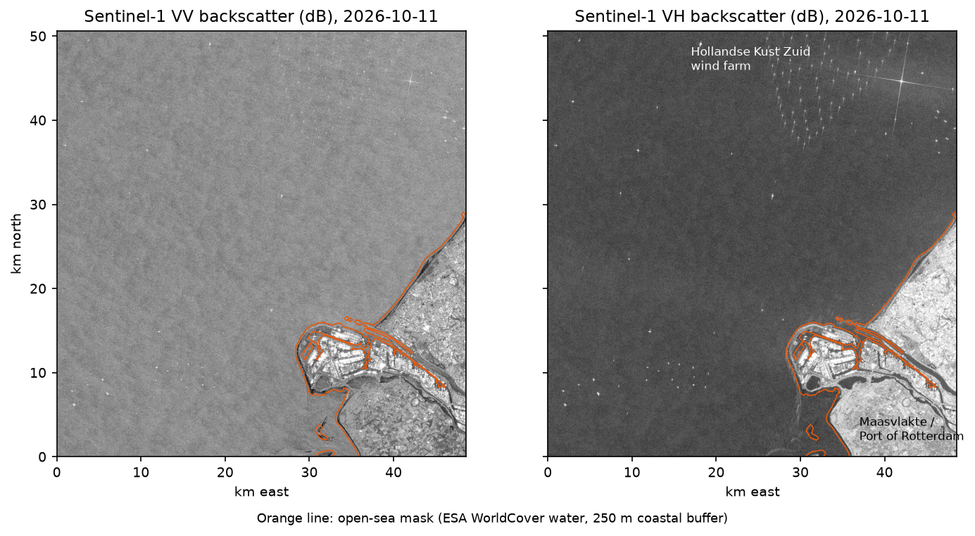

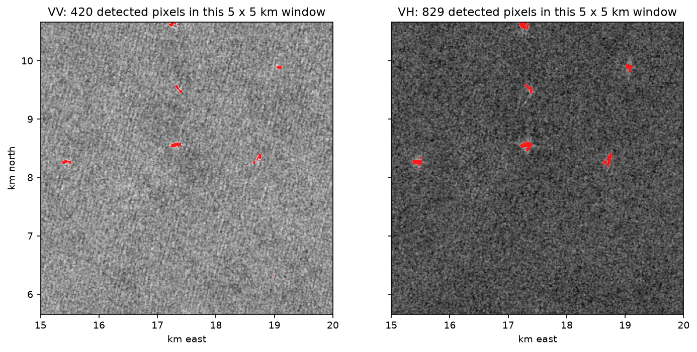
Look at the two images side by side. The sea is about 15 dB darker in VH than in VV, but ships and turbines are bright in both. This difference is why VH is popular for ship detection.

Step 3: a CA-CFAR detector in NumPy and SciPy

A fixed threshold does not work at sea. Sea brightness changes with wind speed, wind direction and incidence angle, and a threshold that is right in calm water will flag every wave in a gale. CFAR solves this by comparing each pixel with its own neighbourhood.

Cell-averaging CFAR uses three windows around the pixel under test:

• the guard window (here 410 m square) is ignored, so that a ship does not raise its own background estimate;
• the background window (1,010 m square) minus the guard window forms a ring, whose mean is the local clutter level;
• the pixel is a detection if its intensity is more than k times the clutter mean.

Summing a window around every pixel sounds slow, but ndimage.uniform_filter does it for the whole image in milliseconds. The sum over the ring is the big box minus the small box. To handle the coast, we sum the sea pixels and count them separately, and divide; this is a normalised convolution, so land pixels never enter the background.

PFA = 1e-6                          # design probability of false alarm per pixel
GUARD, BACKGROUND = 41, 101         # CFAR window sizes in pixels (410 m guard, 1,010 m background)


def ca_cfar(img: np.ndarray, sea: np.ndarray, pfa: float = PFA, enl: float = ENL):
    """Cell-averaging CFAR. The clutter mean comes from a ring of sea pixels between the guard
    and background windows; the multiplier comes from a gamma model of multilook speckle."""
    x = np.where(sea, np.nan_to_num(img), 0).astype("float64")
    m = sea.astype("float64")
    box_sum = lambda a, k: ndimage.uniform_filter(a, k, mode="constant") * k * k
    n_ring = box_sum(m, BACKGROUND) - box_sum(m, GUARD)
    with np.errstate(divide="ignore", invalid="ignore"):
        clutter = (box_sum(x, BACKGROUND) - box_sum(x, GUARD)) / n_ring
    factor = stats.gamma.isf(pfa, a=enl, scale=1 / enl)   # P(I > factor * mean) = pfa for gamma clutter
    ok = sea & (n_ring > 0.5 * (BACKGROUND ** 2 - GUARD ** 2))
    return ok & (img > factor * clutter), clutter, factor


det_vv, clutter_vv, factor = ca_cfar(vv, sea)
det_vh, clutter_vh, _ = ca_cfar(vh, sea)

Where does k come from? In a multilook SAR image of a uniform surface, intensity divided by its mean follows a gamma distribution with shape and rate equal to the ENL. So stats.gamma.isf(pfa, a=ENL, scale=1/ENL) gives the multiplier that pure speckle exceeds with probability pfa. The detector works in linear intensity, never in decibels.

Pfa 1e-06, ENL 4.4: threshold = 5.04 x local clutter mean (7.0 dB above it)
background ring 410 m to 1010 m wide; expected false-alarm pixels over pure gamma speckle: 21
detected pixels: VV 9,984, VH 25,941
VV: sea clutter median -9.6 dB; isolated speckle hits (clusters < 4 px) 623 = 2.9e-05 of sea pixels
VH: sea clutter median -25.1 dB; isolated speckle hits (clusters < 4 px) 892 = 4.2e-05 of sea pixels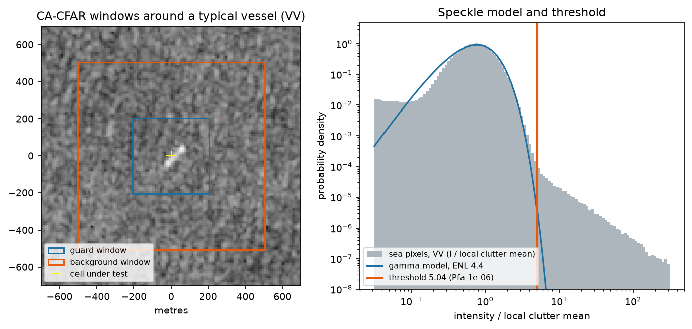

The histogram shows the main weakness of the simple model. Near the mean, the real sea matches the gamma curve well. In the tail, it does not. Real sea clutter is spikier than pure speckle because of waves and swell, and the 10 m RTC pixels are smaller than Sentinel-1’s actual resolution of about 20 m, so neighbouring pixels are correlated. As a result, isolated speckle crossed the threshold about 30 to 40 times more often than designed (2.9 × 10⁻⁵ in VV against 10⁻⁶). Almost all of those false hits are single pixels or pairs, so the next step removes them by size. Heavier-tailed models, such as the K-distribution or a generalised gamma, give more accurate thresholds.

Step 4: cluster the detections into targets

A ship is not one pixel. A 300 m container ship lights up dozens of pixels, often in several fragments. We label connected detections in VV or VH with ndimage.label, measure each blob, and then merge blobs whose centroids are within 250 m of each other into one target. The merge uses a k-d tree to find close pairs and a sparse graph to find connected groups. Targets smaller than 4 pixels (400 m²) are dropped as speckle.

MIN_PIXELS = 4                      # smallest target kept: 4 pixels = 400 m²
MERGE = 250                         # blobs closer than this (m) are one target


def targets(det_a, det_b, img_a, img_b, clut_a, clut_b) -> pd.DataFrame:
    """Label connected detections in either polarisation, then merge blobs closer than MERGE metres."""
    det = det_a | det_b
    lab, n = ndimage.label(det, structure=np.ones((3, 3)))
    idx = np.arange(1, n + 1)
    rows, cols = np.indices(det.shape)
    ratio = np.where(det, np.nan_to_num(img_a / clut_a) + np.nan_to_num(img_b / clut_b), 0)
    tot = ndimage.sum(ratio, lab, idx)
    sl = ndimage.find_objects(lab)
    blobs = pd.DataFrame({
        "row": ndimage.sum(ratio * rows, lab, idx) / tot, "col": ndimage.sum(ratio * cols, lab, idx) / tot,
        "pixels": ndimage.sum(det, lab, idx), "in_a": ndimage.maximum(det_a, lab, idx).astype(bool),
        "in_b": ndimage.maximum(det_b, lab, idx).astype(bool),
        "extent_m": [RES * np.hypot(s[0].stop - s[0].start, s[1].stop - s[1].start) for s in sl],
        "tcr_a": to_db(ndimage.maximum(np.where(det, img_a / clut_a, 0), lab, idx)),
        "tcr_b": to_db(ndimage.maximum(np.where(det, img_b / clut_b, 0), lab, idx)),
        "peak_a": to_db(ndimage.maximum(np.where(det, img_a, 0), lab, idx)),
        "peak_b": to_db(ndimage.maximum(np.where(det, img_b, 0), lab, idx))})
    links = cKDTree(blobs[["row", "col"]] * RES).query_pairs(MERGE, output_type="ndarray")
    graph = coo_matrix((np.ones(len(links)), (links[:, 0], links[:, 1])), shape=(n, n))
    blobs["target"] = connected_components(graph, directed=False)[1]
    blobs["score"] = blobs[["tcr_a", "tcr_b"]].max(axis=1)
    first = blobs.sort_values("score", ascending=False).groupby("target")
    df = first.first()
    df["pixels"] = first.pixels.sum()
    df["blobs"] = first.size()
    df["in_a"], df["in_b"] = first.in_a.any(), first.in_b.any()
    df = df[df.pixels >= MIN_PIXELS].reset_index(drop=True)
    df["x"], df["y"] = x0 + (df.col + 0.5) * RES, y1 - (df.row + 0.5) * RES
    return df.rename(columns={"in_a": "in_vv", "in_b": "in_vh", "tcr_a": "tcr_vv_db", "tcr_b": "tcr_vh_db",
                              "peak_a": "peak_vv_db", "peak_b": "peak_vh_db"}).drop(columns=["score"])


t = targets(det_vv, det_vh, vv, vh, clutter_vv, clutter_vh)

Each target keeps the position of its brightest blob, the total number of detected pixels, whether it was seen in VV and in VH, and its target-to-clutter ratio (TCR): how many decibels its peak is above the local sea.

1,251 connected blobs in VV or VH -> 208 targets after merging blobs within 250 m and dropping those under 4 pixels
seen in both 144, VV only 19, VH only 45
median target-to-clutter ratio of targets seen in both: VV 16.6 dB, VH 23.2 dB

From 1,251 raw blobs, we have 208 targets. The size filter removed most of the speckle hits. For targets seen in both polarisations, VH gives 6.6 dB more contrast than VV, because the sea is so dark in cross-polarisation.

Step 5: sidelobes and azimuth ambiguities

Not every bright spot at sea is a separate object. Two radar artefacts cause most false alarms around very bright targets.

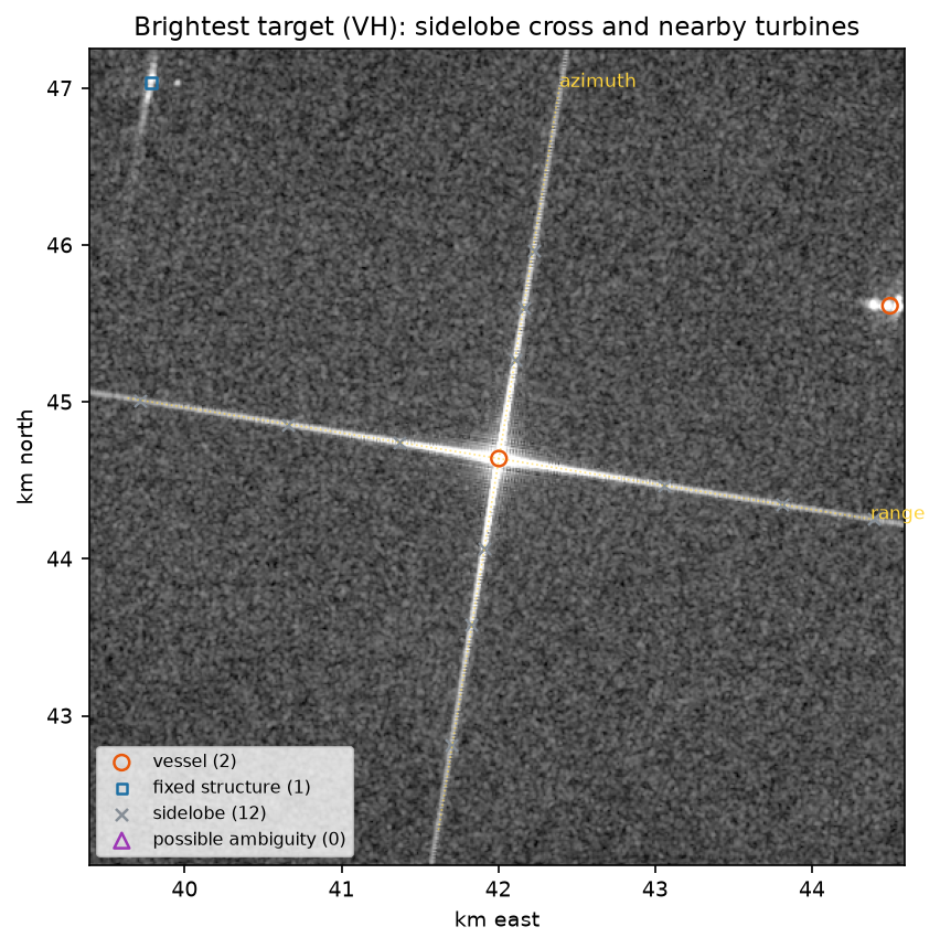
Sidelobes. SAR focusing spreads a little of every target’s energy along two lines through it: one in the range direction (across the flight path) and one in the azimuth direction (along it). Around an extremely bright target, these sidelobes form a cross several kilometres long, and CFAR detects the brighter parts of it as a chain of small targets.

Azimuth ambiguities. The radar samples the Doppler spectrum at its pulse repetition frequency (PRF), so a very bright target also produces faint ghost copies displaced along the azimuth direction by about λ · R · PRF / (2V). For Sentinel-1 IW, with a slant range R of about 850 km, a PRF of about 1,450–1,720 Hz and a velocity V of about 7.6 km/s, that is roughly 4.5–5.3 km. We search a slightly wider band of 4–6.5 km.

To flag either, we need the azimuth and range directions on our UTM grid. Rather than computing them from the orbit, we measure them from the image: the brightest target’s sidelobe cross is a perfect compass. We sample the image along lines through it at every angle and take the brightest line.

AMB_KM = (4.0, 6.5)                 # azimuth ambiguity offset band for IW mode


def arm_angle(img: np.ndarray, r: float, c: float) -> float:
    """Bearing (degrees clockwise from grid north) of the brightest straight arm through pixel (r, c)."""
    db = np.nan_to_num(to_db(img), nan=-40)
    s = np.arange(150, 2500, RES) / RES                  # sample 150 m to 2.5 km either side, in pixels
    angles = np.arange(0, 180, 0.25)
    score = [ndimage.map_coordinates(db, [np.r_[r - s * np.cos(a), r + s * np.cos(a)],
                                          np.r_[c + s * np.sin(a), c - s * np.sin(a)]], order=1).mean()
             for a in np.radians(angles)]
    return float(angles[int(np.argmax(score))])


bright = t.loc[t.tcr_vh_db.idxmax()]
a1 = arm_angle(vh, bright.row, bright.col)
AZ = min((a1, (a1 + 90) % 180), key=lambda a: min(a, 180 - a))   # the arm closest to north-south
u_az = np.array([np.sin(np.radians(AZ)), np.cos(np.radians(AZ))])
u_rg = np.array([u_az[1], -u_az[0]])


def flag_artefacts(df: pd.DataFrame) -> pd.DataFrame:
    xy = df[["x", "y"]].to_numpy()
    pk = df[["peak_vv_db", "peak_vh_db"]].to_numpy()
    side, amb = np.zeros(len(df), bool), np.zeros(len(df), bool)
    for k in range(len(df)):
        d = xy - xy[k]
        along, across = np.abs(d @ u_az), np.abs(d @ u_rg)
        brighter = np.any(pk > pk[k] + 10, axis=1)          # 10 dB brighter in VV or VH
        on_arm = ((along < 3000) & (across < 60)) | ((across < 3000) & (along < 60))
        side[k] = np.any(brighter & on_arm)
        amb[k] = np.any(brighter & (along > AMB_KM[0] * 1000) & (along < AMB_KM[1] * 1000) & (across < 300))
    return df.assign(sidelobe=side, ambiguity=amb & ~side)


t = flag_artefacts(t)

brightest target: VH 54.1 dB above clutter at row 602, col 4200
its sidelobe cross gives azimuth 9.2° and range 99.2° (grid bearings)
azimuth ambiguity offset lambda*R*PRF/(2V) for IW: 4.0-6.5 km
targets on the sidelobe cross of one >= 10 dB brighter: 35
targets at the ambiguity offset of one >= 10 dB brighter: 6

The azimuth direction of 9.2° (and 189.2°) matches a descending Sentinel-1 pass, which flies south-south-west. A target is flagged as a sidelobe if it lies within 60 m of the cross of a target at least 10 dB brighter, and as a possible ambiguity if it sits 4–6.5 km along the azimuth direction from one. That removed 35 sidelobe detections and 6 possible ambiguities.

Step 6: fixed structures persist, ships move

The biggest source of false “ships” here is the wind farm. A wind turbine is a steel tower on the sea: to a radar, it looks just like a small ship. Oil and gas platforms, large navigation buoys and met masts behave the same way.

The difference is that they do not move. We run the same detector on all six passes and count, for each target on 11 October, on how many of the other five passes there was a target within 100 m. A target present on at least four of them is classed as a fixed structure.

FIXED_M = 100                       # within this distance on another pass = the same object

per_date = {MAIN_DATE: t}
for d in DATES:
    if d not in per_date:
        a, b = read_date(d, "vv"), read_date(d, "vh")
        ok = sea & np.isfinite(a) & np.isfinite(b)
        (da, ca, _), (db_, cb, _) = ca_cfar(a, ok), ca_cfar(b, ok)
        per_date[d] = flag_artefacts(targets(da, db_, a, b, ca, cb))
others = [d for d in DATES if d != MAIN_DATE]
t["dates_seen"] = sum((cKDTree(per_date[d][["x", "y"]]).query(t[["x", "y"]], distance_upper_bound=FIXED_M)[0]
                       < FIXED_M).astype(int) for d in others)
t["fixed"] = t.dates_seen >= len(others) - 1        # there on (almost) every other pass
t["class"] = np.select([t.sidelobe, t.ambiguity, t.fixed], ["sidelobe", "possible ambiguity", "fixed structure"],
                       "vessel")

5 other passes; main-date targets also found within 100 m on n other passes: {0: 94, 1: 18, 2: 7, 3: 7, 4: 6, 5: 76}
class
vessel                87
fixed structure       80
sidelobe              35
possible ambiguity     6

The histogram of dates_seen is strongly bimodal. 94 targets appeared only on this pass, which is what you expect for ships under way. 76 targets were there on every pass: those are fixed. The few in between are ships that stayed at anchor for a week or two, and edge cases.

To check the fixed structures independently, the script downloads the offshore wind turbines mapped in OpenStreetMap inside the box from the Overpass API:

64 OSM wind turbines over open sea in the box; 100% have a target within 100 m (median offset 39 m)
fixed structures within 100 m of an OSM turbine: 63 of 80

Every one of the 64 mapped turbines in the box was detected, with a median position error of 39 m. 63 of our 80 fixed structures are those turbines. The other 17 are persistent targets that are not mapped as turbines. Some lie along the Maasgeul approach channel, where large navigation buoys are a likely explanation; others may be platforms or ships that stayed anchored for the whole period. We cannot tell which from radar alone.

Step 7: export the vessels and count them per pass

Finally, we convert the target positions to longitude and latitude and write every target, with its class and measurements, to a GeoJSON file. Keeping all the targets, rather than only vessels, lets you filter them in QGIS or GeoPandas later.

lon, lat = to_lonlat.transform(t.x.to_numpy(), t.y.to_numpy())
cols = ["class", "pixels", "blobs", "extent_m", "tcr_vv_db", "tcr_vh_db", "in_vv", "in_vh", "dates_seen"]
gdf = gpd.GeoDataFrame(t[cols].round(1), geometry=gpd.points_from_xy(np.round(lon, 5), np.round(lat, 5)),
                       crs="EPSG:4326")
gdf.to_file(OUT / f"ship_detections_{MAIN_DATE}.geojson", driver="GeoJSON")
ships = gdf[gdf["class"] == "vessel"]

87 vessels written to output/ship_detections_2026-10-11.geojson (all 208 targets kept, with a class column)
vessel extent median 152 m, largest 544 m; seen in VV 82%, in VH 79%, in both 61%
 class  pixels  blobs  extent_m  tcr_vv_db  tcr_vh_db  in_vv  in_vh  dates_seen     lon      lat
vessel   376.0      1     544.5       48.7       54.1   True   True           3 4.16453 52.24682
vessel   482.0      9     495.2       43.0       29.3   True   True           1 3.99061 51.97583
vessel   280.0      3     374.8       41.8       22.5   True   True           0 4.22320 52.20756
vessel   417.0      6     389.0       38.7       33.0   True   True           1 3.57532 51.90549
vessel   227.0      9     330.2       35.9       31.8   True   True           0 4.25611 52.19563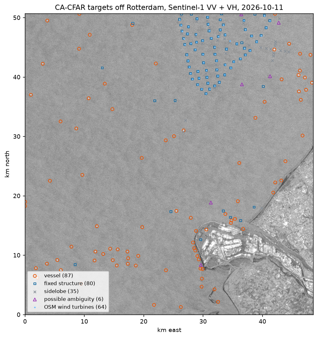

The map tells a clear story. Vessels gather in the anchorage areas west of the Maasvlakte and queue along the approach to the harbour entrance. The turbines of Hollandse Kust Zuid form a regular grid in the north, and the sidelobe crosses sit around the brightest targets there.

Counting every pass the same way shows how busy these waters are:

      date    platform  targets  fixed  artefacts  vessels
2026-09-05 sentinel-1c      239     79         48      112
2026-09-11 sentinel-1d      250     75         30      145
2026-09-17 sentinel-1c      258     79         48      131
2026-09-23 sentinel-1d      305     79         54      172
2026-09-29 sentinel-1c      349     78        103      168
2026-10-11 sentinel-1c      208     80         41       87
mean 136 vessels per pass, range 87-172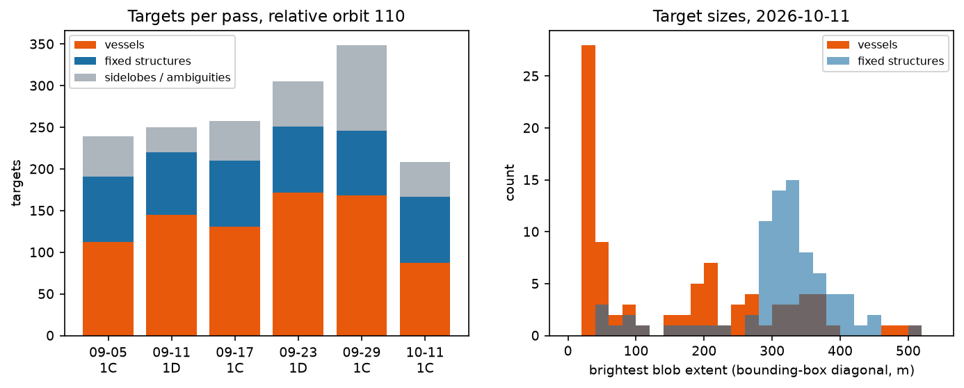

The count of fixed structures is almost constant at 75–80 on every pass, which is reassuring: the same turbines are detected each time. The vessel count varies from 87 to 172 between passes, and the number of artefacts varies even more, from 30 to 103. It rises when there are more very bright targets in the scene and when the sea is rougher.

The size histogram also carries a warning. The extent of a blob is not the length of a ship. Bright targets spread their energy into sidelobes and blur, so turbine blobs measure 300–400 m even though a tower is only a few metres wide. Estimating ship length from SAR needs a tighter threshold on each target or a model trained on known ships.

Limitations and false positives

• No ground truth here. We did not compare the detections with AIS (the Automatic Identification System that ships broadcast), so we cannot give a detection rate or a false-alarm rate per ship. Public AIS archives, such as those of national maritime authorities or Global Fishing Watch, make that possible. Without AIS, treat the vessel count as an estimate.
• Fixed structures. Wind turbines, platforms, buoys and met masts look like ships. Persistence across passes works well, but it needs several dates and it fails for ships that stay at anchor for weeks. A map of known structures, such as OpenStreetMap or the national offshore infrastructure registers, can be used as a mask instead.
• Artefacts. Sidelobes and azimuth ambiguities appear around very bright targets. Our geometric filters are simple; operational systems also check the expected ambiguity brightness from the radar’s antenna pattern.
• Small boats and wooden or fibreglass hulls reflect little, and in rough seas they disappear into the clutter. Sentinel-1 IW at about 20 m resolution reliably detects ships longer than about 25–50 m, depending on the wind.
• Sea state. Strong wind, breaking waves, rain cells and current fronts raise the clutter and its tail. CFAR adapts to the mean, but our gamma model underestimates the tail, so false alarms rise in rough seas. A K-distribution or a two-parameter CFAR helps.
• Coasts and harbours. The 250 m buffer removes ships moored alongside and in harbour basins, which are often the majority in port. Those need very-high-resolution imagery or AIS.

Frequently asked questions

Can Sentinel-1 detect ships?

Yes. Ships are strong radar reflectors, and Sentinel-1 images the sea day and night through cloud. Its Interferometric Wide swath mode covers 250 km at about 20 m resolution, which is enough to detect most ships longer than a few tens of metres. Sentinel-1 data is free, and it is used operationally, for example by the European Maritime Safety Agency.

What is a CFAR detector?

CFAR stands for constant false alarm rate. Instead of one fixed threshold, a CFAR detector sets the threshold for each pixel from the statistics of the background around it, so that the probability of a false alarm stays the same in calm and rough water. Cell-averaging CFAR (CA-CFAR), used in this tutorial, estimates the background as the mean of a ring of pixels around the pixel under test.

Is VV or VH better for ship detection?

VH is usually better, because the sea is much darker in cross-polarisation while ships remain bright. Here, VH gave ships 6.6 dB more contrast. VV still detected some targets that VH missed, and in very calm seas the VH background can fall to the instrument noise floor. Using both polarisations together is the most robust approach.

How do I remove false positives from SAR ship detection?

Mask the land with a buffer, drop targets smaller than a few pixels, and flag targets that persist at the same position across passes, since those are fixed structures such as wind turbines and platforms. Then flag sidelobes along the range and azimuth directions of very bright targets, and azimuth ambiguities several kilometres along track. Finally, compare with AIS data where available.

What are azimuth ambiguities in SAR?

They are faint ghost images of very bright targets, displaced along the satellite’s flight direction. They occur because the radar samples the Doppler spectrum of each target at its pulse repetition frequency, and energy outside that band folds back to a different position. For Sentinel-1 IW, the ghosts appear a few kilometres away along track, and they are typically 20 dB or more fainter than the real target.

Can SAR ship detection find dark ships?

It can find ships that have switched off their AIS transponder, which is why SAR is used to monitor illegal fishing and sanctions evasion. Matching SAR detections with AIS positions shows which vessels are broadcasting and which are not. This tutorial does not do that matching, so it cannot identify any ship as dark.

Next steps

• Add public AIS data for the same times and measure the detection rate and false alarms per vessel.
• Replace the gamma threshold with a K-distribution CFAR, and compare the false-alarm rates.
• Estimate ship length and heading from each target’s chip, or train a small classifier on the chips.
• Map water instead of ships in Sentinel-1 SAR flood mapping in Python, or measure millimetres of ground motion from the same satellite’s phase in InSAR ground subsidence in Python.
• Load the GeoJSON into GeoPandas and map it interactively with Folium.

Data and licences

• Sentinel-1 RTC: contains modified Copernicus Sentinel data 2026, processed by ESA; radiometric terrain correction by Catalyst/Microsoft. Licensed CC BY 4.0. Accessed from the Microsoft Planetary Computer in October 2026.
• ESA WorldCover 2021 v200: © ESA WorldCover project 2021, contains modified Copernicus Sentinel data processed by the ESA WorldCover consortium. Licensed CC BY 4.0. Accessed from the Microsoft Planetary Computer.
• OpenStreetMap: wind turbine positions © OpenStreetMap contributors, available under the Open Database Licence (ODbL), queried through the Overpass API.
• Code: ship_detection_cfar.py, tested with Python 3.12.0, pystac-client 0.9.0, planetary-computer 1.0.0, rasterio 1.5.2, SciPy 1.18.1 and GeoPandas 1.2.0.