Sentinel-1 crop monitoring in Python: SAR time series for wheat and oilseed rape

Short answer: to monitor crops with Sentinel-1 in Python, search the Planetary Computer’s sentinel-1-rtc collection for one relative orbit across the season. Stream the VV and VH bands onto a common grid, then average the linear backscatter over each field to remove speckle, and only then convert to decibels. Plot VV, VH and the VH/VV ratio (VH dB − VV dB) per crop. A growing canopy raises VH and the ratio. Oilseed rape, winter wheat and spring crops each leave a distinct curve, and the radar records it every 12 days whatever the weather.

England’s arable east is cloudy for much of the year. An optical satellite such as Sentinel-2 often fails to see a field for weeks, and the gap tends to fall in spring, just when crops grow fastest. Radar sees through cloud. In this tutorial, we follow 247 fields between Royston and Cambridge through the 2024 harvest year with free Sentinel-1 data. We label them with the open Crop Map of England and measure how many usable Sentinel-2 views the same fields got.

You will learn how to:

1. get field boundaries from OpenStreetMap and crop labels from CROME 2024 through its OGC API;
2. stream a season of Sentinel-1 RTC from one orbit and average it per field;
3. measure speckle, and see why field-averaging beats filtering for this job;
4. read the VV, VH and VH/VV ratio growth signatures of winter wheat, oilseed rape, spring barley and maize;
5. count the Sentinel-2 cloud gaps over the same fields and compare NDVI with the radar ratio;
6. test how well the radar time series alone separates the crops.

All outputs below are real results from s1_crop_monitoring.py, run on 17 October 2026 with Python 3.12, pystac-client 0.9.0, rasterio 1.5.2 and osmnx 2.1.1. A full run takes about a minute on a home broadband connection.

Why radar for agriculture?

Sentinel-1 carries a C-band synthetic aperture radar with a 5.6 cm wavelength. It makes its own illumination, so it images at night, and it passes through cloud. What comes back from a field depends on the soil’s roughness and moisture and on the size, shape, water content and orientation of the plants.

• VV (vertical send, vertical receive) responds strongly to the soil surface and to vertical stems. A dense, upright cereal canopy attenuates VV, so VV falls as wheat grows tall.
• VH (vertical send, horizontal receive) comes mostly from volume scattering: the pulse bounces around among leaves, branches and pods, which depolarises it. VH rises with biomass, especially for broad-leaved, branching crops such as oilseed rape.
• The VH/VV ratio cancels some of the effect of soil moisture and incidence angle that both bands share. It tracks canopy development closely, which is why it is often compared with NDVI.

If you are new to SAR, start with Sentinel-1 SAR flood mapping in Python, which covers decibels, speckle and orbits in more detail.

Step 1: field boundaries from OpenStreetMap

We need field polygons to average over. In much of rural England, OpenStreetMap volunteers have mapped farmland as landuse=farmland. Some polygons are single fields; others cover several. We fetch them with OSMnx, keep those of 3–100 ha, and shrink each by 20 m. That drops hedges, tracks and the mixed pixels at the field edge.

BBOX = (-0.12, 52.08, 0.02, 52.17)    # lon/lat: arable South Cambridgeshire, between Royston and Cambridge
CRS = "EPSG:32630"                    # UTM zone 30N: the native grid of these Sentinel-1 and Sentinel-2 scenes
INSET_M = 20                          # shrink each field by 20 m to drop hedges, tracks and mixed edge pixels

osm = ox.features_from_bbox(BBOX, {"landuse": "farmland"})
fields = osm[osm.geometry.type.isin(["Polygon", "MultiPolygon"])].reset_index().to_crs(CRS)
aoi_utm = gpd.GeoSeries([box(*BBOX)], crs=4326).to_crs(CRS).iloc[0]
fields = fields[fields.within(aoi_utm)].copy()
fields["area_ha"] = fields.area / 1e4
fields["core"] = fields.buffer(-INSET_M)
fields = fields[(fields["area_ha"] >= 3) & (fields["area_ha"] <= 100) & ~fields["core"].is_empty].reset_index(drop=True)

The script saves the result to a GeoPackage and retries a second Overpass server if the first is busy, so you only download the polygons once.

413 polygons of 3-100 ha inside the study area, median 10.5 ha, total 5,636 ha

Step 2: crop labels from the Crop Map of England

To know which signature belongs to which crop, we need labels. The Rural Payments Agency publishes the Crop Map of England (CROME) every year under the Open Government Licence. It is a grid of hexagons of about 0.4 ha, each with a crop code. The 2024 map is available through an OGC API – Features endpoint, which returns GeoJSON in pages of up to 10,000 features:

CROME = ("https://environment.data.gov.uk/spatialdata/crop-map-of-england-2024/ogc/features/v1/"
         "collections/Crop_Map_of_England_2024_Cambridgeshire/items")
CROPS = {"AC66": "Winter wheat", "AC67": "Winter oilseed rape", "AC63": "Winter barley", "AC01": "Spring barley",
         "AC17": "Maize", "AC03": "Sugar beet", "LG20": "Winter field beans", "PG01": "Grass",
         "TG01": "Temporary grass", "FA01": "Fallow"}
MIN_HEX, MIN_PURITY = 10, 0.8          # a field needs >= 10 CROME hexagons, and >= 80% of them must agree

feats, url = [], CROME
params = {"f": "json", "limit": 10000, "bbox": ",".join(map(str, BBOX))}
while url:                                  # OGC API Features: follow the "next" links page by page
    r = requests.get(url, params=params, timeout=300)
    r.raise_for_status()
    page = r.json()
    feats += page["features"]
    url, params = next((lk["href"] for lk in page.get("links", []) if lk["rel"] == "next"), None), None
hexes = gpd.GeoDataFrame.from_features(feats, crs=4326).to_crs(CRS)
hexes["geometry"] = hexes.centroid
joined = gpd.sjoin(hexes, fields.set_geometry("core")[["core"]], predicate="within")
stats = joined.groupby("index_right")["lucode"].agg(n_hex="size", lucode=lambda s: s.mode().iloc[0],
                                                     purity=lambda s: s.value_counts(normalize=True).iloc[0])
fields = fields.join(stats)
fields["crop"] = fields["lucode"].map(CROPS).fillna("Other")
labelled = fields[(fields["n_hex"] >= MIN_HEX) & (fields["purity"] >= MIN_PURITY)].reset_index(drop=True)

We give each OSM polygon the most common CROME code among the hexagons inside it. We keep it only if at least 80% of the hexagons agree. That drops polygons that span several fields with different crops.

24,734 CROME hexagons; 413 polygons contain hexagons
247 fields are >= 80% one crop (the rest are mixed, or the OSM polygon spans several fields)
                     fields  median_ha
crop
Winter wheat            129       12.2
Spring barley            35       13.0
Winter oilseed rape      21       14.7
Winter barley            18       15.5
Grass                    13        9.8
Winter field beans        8        8.5
Maize                     8       15.2
Sugar beet                6       13.1
Fallow                    4       15.0
Other                     4        7.0
Temporary grass           1        7.0

Step 3: a season of Sentinel-1 RTC, averaged per field

The Planetary Computer’s sentinel-1-rtc collection already has terrain-corrected backscatter (γ⁰) as Cloud Optimised GeoTIFFs. Over this area, four relative orbits pass: two ascending and two descending. Each sees the fields from a different angle, and backscatter depends on the angle, so we keep one orbit. Orbit 59 passes at about 18:00 UTC, heading north.

The 2024 harvest year starts in September 2023, when winter crops are sown:

SEASON = "2023-09-01/2024-09-30"      # the 2024 harvest year: winter crops are sown in autumn 2023
ORBIT = 59                            # one relative orbit (ascending, ~18:00 UTC): identical geometry every 12 days

catalog = pystac_client.Client.open(STAC_URL, modifier=planetary_computer.sign_inplace)
search = catalog.search(collections=["sentinel-1-rtc"], bbox=BBOX, datetime=SEASON,
                        query={"sat:relative_orbit": {"eq": ORBIT}})
s1_items = sorted(search.items(), key=lambda i: i.datetime)

33 scenes from relative orbit 59 (ascending), 04 Sep 2023 to 22 Sep 2024
platforms: {'SENTINEL-1A': 33}
example: S1A_IW_GRDH_1SDV_20230904T174210_20230904T174235_050181_060A2D_rtc | polarisations ['VV', 'VH']

We rasterise the shrunken field cores onto a 10 m grid in UTM zone 30N. For each scene, we stream VV and VH onto that grid with a WarpedVRT and sum the pixels per field with scipy.ndimage.sum. The key detail is that we average linear power, never decibels: the mean of logarithms is not the logarithm of the mean.

labels = rasterio.features.rasterize(zip(labelled["core"], labelled["fid"]), out_shape=(HEIGHT, WIDTH),
                                     transform=TRANSFORM, fill=0, dtype="int32")
FIDS = labelled["fid"].to_numpy()
npix = ndimage.sum(np.ones_like(labels), labels, FIDS)


def field_means(img: np.ndarray) -> np.ndarray:
    """Mean of the valid (non-NaN) pixels in each field core. Use it on linear power, never on dB."""
    ok = np.isfinite(img)
    s = ndimage.sum(np.where(ok, img, 0), labels, FIDS)
    n = ndimage.sum(ok, labels, FIDS)
    with np.errstate(invalid="ignore", divide="ignore"):
        return np.where(n >= 0.8 * npix, s / n, np.nan)   # need 80% of the field core covered


def s1_scene(item) -> dict:
    out = {}
    for pol in ("vv", "vh"):
        g0 = read_warped(item.assets[pol].href)  # WarpedVRT onto the 10 m grid, average resampling
        g0[g0 <= 0] = np.nan
        out[pol] = field_means(g0)
    return {"date": item.datetime, **out}


with ThreadPoolExecutor(max_workers=8) as pool:
    scenes = list(pool.map(s1_scene, s1_items))
VV = np.array([s["vv"] for s in scenes])             # dates x fields, linear power
VH = np.array([s["vh"] for s in scenes])

The full script also caches each scene to a small .npz file and keeps three full images for the maps.

1000 x 1040 pixels of 10 m (10.0 x 10.4 km), EPSG:32630
field cores: median 941 pixels per field (min 343, max 5119)
read and field-averaged 33 scenes x 2 polarisations in 12 s

Reading 66 rasters takes 12 seconds because rasterio fetches only the part of each Cloud Optimised GeoTIFF that covers our 10 km box.

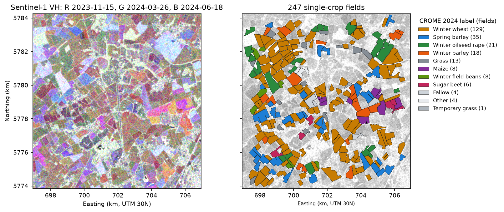
The colour composite already separates crops. Oilseed rape is bright in VH all spring, so it shows as white or pale green. Spring crops are bare in November and March, and their canopy grows by June, so they look blue. Wheat looks dark red to brown.

Step 4: speckle, and why we average per field

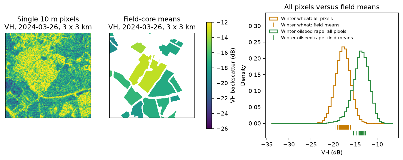
Each Sentinel-1 pixel is speckled: random interference between scatterers makes neighbouring pixels in the same field differ by several decibels. In the flood tutorial we used a Lee filter, because we needed a map of every pixel. For crop monitoring we want one number per field, so we can simply average all the pixels in it. How good is that average? A split-half test tells us: put each pixel at random into half A or half B, average each half, and compare.

inside = labels > 0
pix_db = db(vh_img[inside])
lab_in = labels[inside]
within_std = pd.Series(pix_db).groupby(lab_in).std()
rng = np.random.default_rng(0)
half = rng.random(inside.sum()) < 0.5          # split each field's pixels at random into two halves
lin = vh_img[inside]
mean_a = pd.Series(lin[half]).groupby(lab_in[half]).mean()
mean_b = pd.Series(lin[~half]).groupby(lab_in[~half]).mean()
half_diff = (db(mean_a) - db(mean_b)).dropna()

VH on 2024-03-26: median within-field pixel std 1.61 dB
split-half test: std of (half A - half B) = 0.114 dB, so a whole-field mean is good to about 0.057 dB

Each half has a speckle error of about 0.114 / √2 ≈ 0.08 dB. The whole field has twice as many pixels, so its error is about 0.057 dB, nearly 30 times smaller than the 1.6 dB scatter of single pixels. That is far smaller than the 5–8 dB changes that crops cause, so no speckle filter is needed once you average per field.

Step 5: crop growth signatures in VV, VH and VH/VV

With a clean time series for each field, we take the median field of each crop on each date and plot the interquartile range around it. The ratio in decibels is just a subtraction:

vv_db, vh_db = db(VV), db(VH)
ratio_db = vh_db - vv_db                       # VH/VV ratio in dB = VH(dB) - VV(dB)
long = pd.DataFrame({
    "date": np.repeat(S1_DATES, len(FIDS)), "fid": np.tile(FIDS, len(S1_DATES)),
    "vv_db": vv_db.ravel(), "vh_db": vh_db.ravel(), "ratio_db": ratio_db.ravel()})
long = long.merge(labelled[["fid", "id", "crop", "area_ha"]].rename(columns={"id": "osm_id"}), on="fid")
long.round(3).to_csv(OUT / "field_backscatter_timeseries.csv", index=False)
med = long.groupby(["crop", "date"])[["vv_db", "vh_db", "ratio_db"]].median()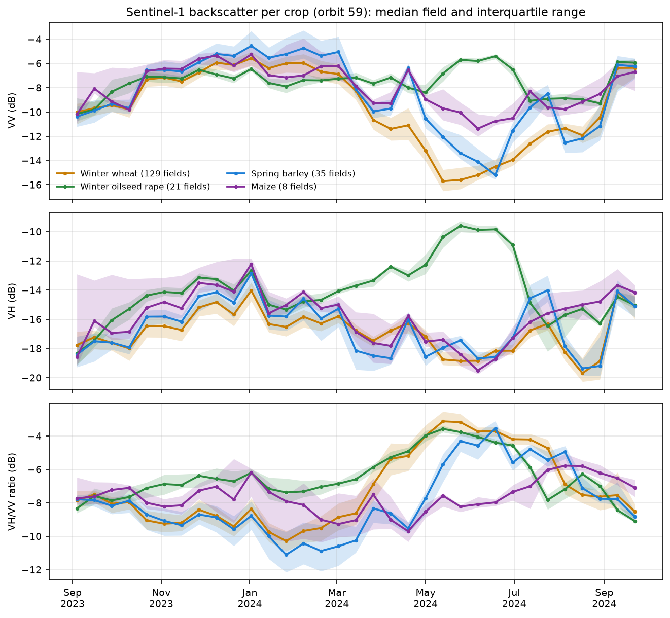

               crop  fields  VH Nov-Dec  VH Mar  VH May-Jun  VV May-Jun  VH/VV May-Jun  VH/VV Sep
       Winter wheat     129       -15.8   -16.7       -18.3       -14.7           -3.7       -8.0
Winter oilseed rape      21       -13.7   -13.7       -10.5        -6.4           -4.1       -8.8
      Spring barley      35       -15.1   -17.3       -18.1       -12.8           -5.2       -8.3
              Maize       8       -14.3   -16.5       -18.1       -10.2           -8.0       -6.8
      Winter barley      18       -16.0   -16.5       -16.2       -11.8           -4.3       -8.2
         Sugar beet       6       -13.9   -18.4       -16.5        -9.7           -6.6       -6.5
 Winter field beans       8       -15.0   -17.3       -13.9        -8.4           -5.4       -8.3
              Grass      13       -16.3   -16.4       -16.2       -11.1           -5.0       -5.7
largest all-field VV jumps: 10 Sep 2024 +3.8 dB, 22 Oct 2023 +2.4 dB, 13 May 2024 -2.3 dB
Winter wheat: VH/VV highest -3.1 dB on 13 May 2024, lowest -10.3 dB on 26 Jan 2024; VV lowest -15.7 dB on 13 May 2024
Winter oilseed rape: VH/VV highest -3.6 dB on 13 May 2024, lowest -9.1 dB on 22 Sep 2024; VV lowest -10.2 dB on 04 Sep 2023

How to read the curves:

• Winter oilseed rape is the easiest crop to recognise. It is drilled in late August and builds a leafy rosette before winter, so its VH is already 2 dB above wheat in November and December (−13.7 against −15.8 dB). In spring it grows into a dense, branching, metre-high canopy of stems, flowers and then pods: a perfect volume scatterer. VH reaches about −10 dB in May and June, 8 dB above wheat. VV stays high too (−6.4 dB). After harvest in July both drop sharply.
• Winter wheat looks like bare soil until March. From April, its stems extend and the vertical, water-filled canopy attenuates VV: VV falls from about −6 to −15.7 dB in mid-May, while VH changes little. The VH/VV ratio therefore climbs from −10.3 dB in late January to −3.1 dB on 13 May. As the crop ripens and dries in July, the ratio falls back, and stubble and cultivation after harvest bring VV back up.
• Spring barley follows the same cereal pattern about a month later: it is sown in March, and its ratio peaks in June.
• Maize is sown in May and grows through the summer, so its ratio rises last, in July and August.

The VV jumps that move all crops together on the same date, such as +3.8 dB on 10 September 2024, are not crop growth. Rain wets the soil, which raises its dielectric constant and its backscatter. This is the main nuisance in SAR crop monitoring, and it is why the ratio, which partly cancels it, is popular. Look for these “every field jumps at once” dates and check them against rainfall records before you interpret a single-date change.

Step 6: how often could Sentinel-2 see the same fields?

Now the optical comparison. We search for every Sentinel-2 L2A acquisition over the area in the same season, whatever its cloud cover. For each, we read the scene classification layer (SCL) at 10 m and count the field pixels classed as vegetation or bare soil (classes 4 and 5). Cloud, cloud shadow, cirrus and unclassified pixels count as unusable. Where at least 20% of the field pixels are clear, we also read red and near-infrared and compute NDVI per field, using only clear pixels.

CLEAR_SCL = [4, 5]            # SCL vegetation, not vegetated. Cloud, shadow, cirrus, unclassified etc. are unusable


def s2_scene(item) -> dict:
    scl = read_warped(item.assets["SCL"].href, Resampling.nearest, nodata=0, dtype="uint8")
    clear = np.isin(scl, CLEAR_SCL)
    covered = float((scl[inside] > 0).mean())
    n_clear = ndimage.sum(clear, labels, FIDS)
    out = {"covered": np.array(covered), "clear_frac": np.array(float(clear[inside].mean())),
           "ndvi": np.full(len(FIDS), np.nan)}
    if out["clear_frac"] >= 0.2:               # only read the 10 m bands when there is something to see
        off = -1000 if float(item.properties["s2:processing_baseline"]) >= 4.0 else 0
        red = read_warped(item.assets["B04"].href, nodata=0) + off
        nir = read_warped(item.assets["B08"].href, nodata=0) + off
        with np.errstate(invalid="ignore", divide="ignore"):
            ndvi = np.where(clear, (nir - red) / (nir + red), np.nan)
        s = ndimage.sum(np.nan_to_num(ndvi), labels, FIDS)
        with np.errstate(invalid="ignore", divide="ignore"):
            out["ndvi"] = np.where(n_clear >= 0.8 * npix, s / n_clear, np.nan)
    return {"date": item.datetime, **out}

The −1000 offset matters: Sentinel-2 products from processing baseline 04.00 (January 2022) onwards add 1000 to every reflectance value, and NDVI is wrong if you forget to remove it.

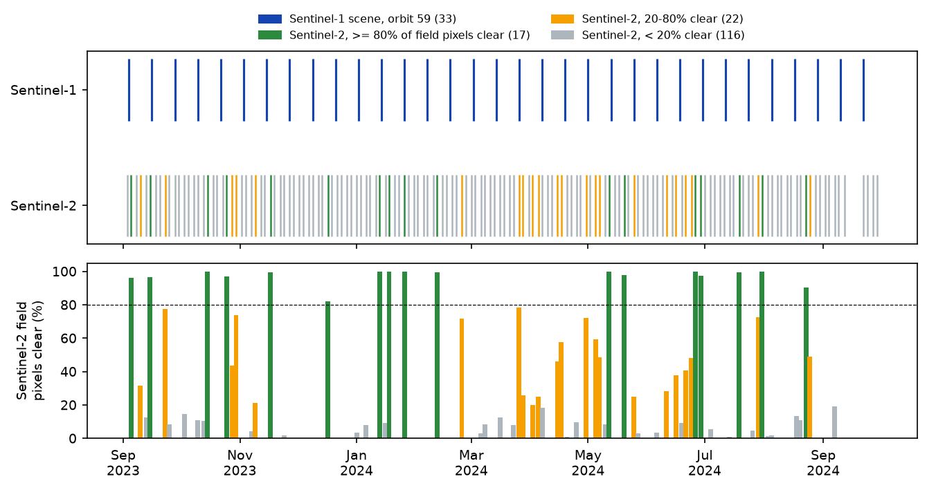
155 Sentinel-2 L2A acquisitions of tile 30UXC (any cloud cover), 03 Sep 2023 to 29 Sep 2024
read SCL (and red/NIR where useful) for 155 acquisitions in 8 s; 155 cover the fields fully
acquisitions with >= 80% of field pixels clear: 17 of 155 (11%)
acquisitions where at least one field is clear: 39
clear NDVI observations per field over 13 months: median 25, min 17, max 31 (Sentinel-1: 33 on every field)
longest gap between clear views of the same field: median 43 days (range 30-90); clear views per field in March-April 2024: median 2
longest gap between >= 80%-clear Sentinel-2 dates: 90 days (12 Feb 2024 to 12 May 2024); longest Sentinel-1 gap: 12 days
          S1 scenes (orbit 59)  S2 acquisitions  S2 >= 80% clear
Sep 2023                     3               12                2
Oct 2023                     2               12                2
Nov 2023                     3               12                1
Dec 2023                     2               12                1
Jan 2024                     3               13                3
Feb 2024                     2               11                1
Mar 2024                     3               13                0
Apr 2024                     2               12                0
May 2024                     3               12                2
Jun 2024                     3               12                2
Jul 2024                     2               13                2
Aug 2024                     3               12                1
Sep 2024                     2                9                0

Sentinel-2A and 2B together visited the area 155 times, about every 2–3 days, but only 17 acquisitions (11%) saw at least 80% of the field area clear of cloud. There was not one such day in March or April 2024, a famously wet spring. The typical field went 43 days without a single clear view, and some went 90 days. Over the same period, Sentinel-1 delivered a clean measurement of every field every 12 days.

Step 7: NDVI and the VH/VV ratio side by side

On the dates when Sentinel-2 can see, how does NDVI compare with the radar? We pair each crop’s median NDVI with the nearest radar date, within three days, and compute a correlation:

for crop in ["Winter wheat", "Winter oilseed rape"]:
    a, b = ndvi_med.loc[crop], med.loc[crop, "ratio_db"]
    pairs = pd.merge_asof(a.rename("ndvi").reset_index().sort_values("date"),
                          b.rename("ratio").reset_index().sort_values("date"),
                          on="date", direction="nearest", tolerance=pd.Timedelta("3D")).dropna()
    r = np.corrcoef(pairs["ndvi"], pairs["ratio"])[0, 1]

Winter wheat: 39 NDVI dates with >= 5 clear fields; 16 within 3 days of a radar date; Pearson r = 0.82
  NDVI outliers (> 0.25 from the 5-date running median): 07 May 2024 (0.15)
Winter oilseed rape: 34 NDVI dates with >= 5 clear fields; 13 within 3 days of a radar date; Pearson r = 0.48
  NDVI outliers (> 0.25 from the 5-date running median): 25 Oct 2023 (0.09), 07 May 2024 (0.21)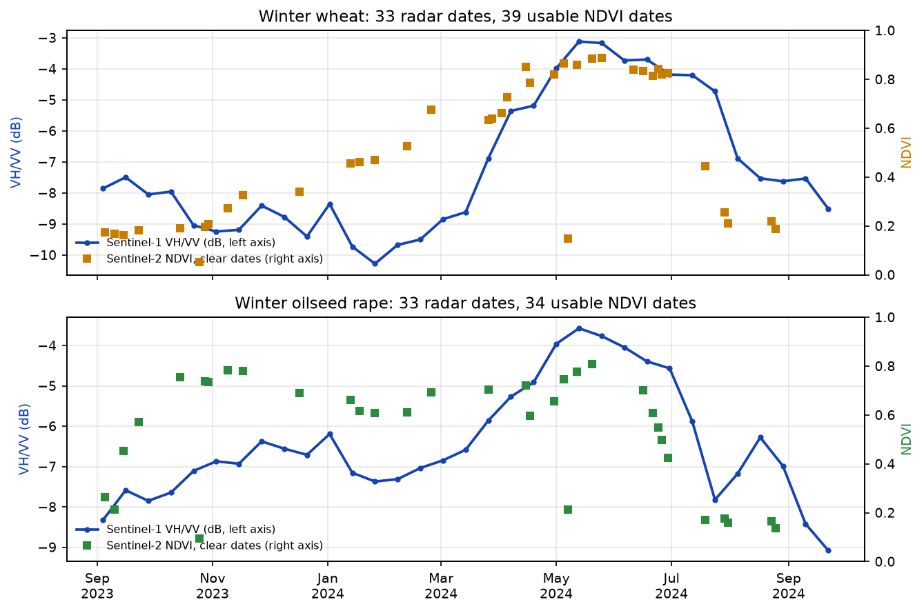

For wheat, the ratio follows NDVI closely (r = 0.82): both track the green canopy from tillering to ripening. For oilseed rape, the agreement is weaker (r = 0.48). Rape is green and leafy from October, so NDVI is high all winter, but the radar ratio rises only when the plants build stems and pods in spring. The two sensors measure different things: NDVI sees chlorophyll, radar sees structure and water. They complement each other rather than one replacing the other.

The outliers are also worth noticing. On 7 May 2024, NDVI over wheat fell to 0.15 between neighbours of about 0.85. Haze or thin cloud that the SCL missed is the likely cause. Cloud masks are not perfect, and radar has no such failure mode.

Step 8: can radar alone tell the crops apart?

As a final test, we try to classify each field from its radar curves alone. We stack the 33 VV and 33 VH values of each field into a 66-number vector and standardise it. Then we assign each field to the crop with the nearest average curve (centroid), computing the centroids without the field being tested (leave-one-out). Crops with fewer than 8 fields are left out.

X = np.hstack([vv_db.T, vh_db.T])[sel]        # fields x (dates x 2) feature matrix
X = (X - X.mean(axis=0)) / X.std(axis=0)
y = labelled.loc[sel, "crop"].to_numpy()
pred = []
for i in range(len(y)):                        # leave one field out, classify it by the nearest class centroid
    keep = np.arange(len(y)) != i
    cents = {c: X[keep][y[keep] == c].mean(axis=0) for c in CLASSES}
    pred.append(min(cents, key=lambda c: np.linalg.norm(X[i] - cents[c])))

219 fields, 66 features (33 dates x VV, VH); overall accuracy 87%
  Winter wheat         recall 86%  (129 fields)
  Winter oilseed rape  recall 100%  (21 fields)
  Winter barley        recall 78%  (18 fields)
  Spring barley        recall 89%  (35 fields)
  Maize                recall 75%  (8 fields)
  Winter field beans   recall 100%  (8 fields)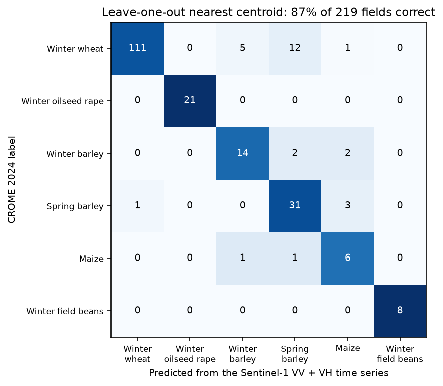

Even this very simple method, with no machine-learning library, matches CROME on 87% of fields and on every oilseed rape and bean field. The main confusion is 12 wheat fields predicted as spring barley: both are cereals with a similar canopy, and late-drilled wheat behaves like a spring crop. A random forest or a temporal neural network on several orbits would do better. That is roughly how CROME itself is made.

Limitations and how to improve them

• One orbit, one angle. We used only orbit 59. Adding the other ascending orbit (132) and the two descending ones (8 and 81) roughly triples the number of dates, but each orbit needs its own reference curves, or a normalisation for incidence angle.
• Soil moisture. Rain moves VV and VH on all fields at once. The ratio helps, but in winter, when there is little canopy, it still follows the weather. Compare with a rainfall series, or use a change-detection approach against neighbouring fields.
• Field boundaries. OSM landuse=farmland polygons often cover several fields. We dropped the mixed ones, which is why only 247 of 413 survived. For production work, use the Rural Payments Agency’s Land Parcels, or segment fields from imagery. The Segment Anything tutorial shows one way.
• Labels from a model. CROME is a classification, not a survey. Some “errors” in Step 8 may be CROME’s.
• Crop calendars vary. Signatures shift with sowing date, variety and weather. Curves from one year and region transfer imperfectly to another.

Frequently asked questions

Can Sentinel-1 be used for crop monitoring?

Yes. Sentinel-1 measures how crops scatter microwaves, which depends on their structure, biomass and water content. With a revisit of 6–12 days that is never interrupted by cloud, it gives a reliable time series for every field, which is ideal for crop type mapping, growth stage monitoring and detecting harvest, ploughing or mowing. It is used operationally in national crop maps, including the Crop Map of England.

What does the VH/VV ratio show for crops?

The VH/VV ratio, VH (dB) minus VV (dB), rises as the canopy grows, because volume scattering from leaves and stems raises VH and a vertical cereal canopy weakens VV. In this tutorial, the median winter wheat field went from −10.3 dB in January to −3.1 dB in mid-May. The ratio is less affected by soil moisture than either band on its own and correlates with NDVI for cereals (r = 0.82 for wheat here).

Why is VH higher for oilseed rape than for wheat?

Oilseed rape grows into a tall, branching canopy of stems, leaves, flowers and pods with many randomly oriented elements. That depolarises the radar pulse and gives strong cross-polarised (VH) backscatter. Wheat stems are mostly vertical and regularly spaced, which attenuates VV rather than adding VH. In May and June 2024, rape fields were about 8 dB brighter in VH than wheat fields (−10.5 against −18.3 dB).

Do I need to filter speckle for crop monitoring?

Not if you average over fields. Average the linear backscatter of all the pixels in a field, then convert the mean to decibels. With about 900 pixels per field, the error from speckle is about 0.06 dB, far below crop effects of several decibels. Use a speckle filter, such as Lee or refined Lee, when you need pixel-level maps instead.

Should I use ascending or descending orbits?

Either, but do not mix them in one time series without care. Ascending and descending passes, and different relative orbits, view the field from different directions and incidence angles, which shifts the backscatter by a decibel or more. Morning (descending) passes over Europe can also see dew on leaves. Start with one orbit, and add others as separate series.

Is Sentinel-1 better than Sentinel-2 for agriculture?

Neither is better; they measure different things. Sentinel-2 NDVI measures greenness directly and is easier to interpret, but in this example it got a clear view of most fields on only 17 of 155 dates. Sentinel-1 never misses a date but is affected by soil moisture and is harder to read. Most operational crop maps use both.

Next steps

• Learn the radar basics, including the Lee filter and decibels, in Sentinel-1 SAR flood mapping in Python.
• Delineate field boundaries yourself with Segment Anything on satellite and aerial imagery.
• Learn STAC and Sentinel-2 cloud masking in Measuring Lake Mead’s shrinking shoreline with Sentinel-2 and STAC and Monitoring reservoir water quality from space with Sentinel-2.
• Add the other three orbits, detect the harvest date of each field from the sudden VH/VV drop, or replace the nearest-centroid classifier with a random forest.
• Compare the radar signatures with an optical view of crop growth in NDVI time series in Python with Sentinel-2 and odc-stac.

Data and licences

• Sentinel-1 RTC: contains modified Copernicus Sentinel data 2023–2024, processed by ESA; radiometric terrain correction by Catalyst/Microsoft. Licensed CC BY 4.0. Accessed from the Microsoft Planetary Computer on 17 October 2026.
• Sentinel-2 L2A: contains modified Copernicus Sentinel data 2023–2024. Accessed from the Microsoft Planetary Computer.
• Crop Map of England (CROME) 2024: © Rural Payments Agency, published by Defra under the Open Government Licence v3.0. Accessed through the Defra Data Services Platform OGC API.
• Field boundaries: © OpenStreetMap contributors, available under the Open Database Licence.
• Code: s1_crop_monitoring.py, tested with Python 3.12.0, pystac-client 0.9.0, planetary-computer 1.0.0, rasterio 1.5.2, geopandas 1.2.0, osmnx 2.1.1 and pandas 3.0.6.