NDVI time series in Python with Sentinel-2, odc-stac and xarray
Build a five-year Sentinel-2 NDVI time series in Python: load a lazy dask datacube with odc-stac, mask cloud with SCL, make monthly composites, extract field curves and derive crop phenology.
- Level
- Intermediate
- Tested with
- Python 3.12
- Source code
- Download scripts
Key takeaways
- odc.stac.load turns a STAC search into a lazy xarray datacube: 396 Sentinel-2 scenes from 2021 to 2025 became a 0.77 GB dask-backed cube in seconds, and nothing was downloaded until .compute().
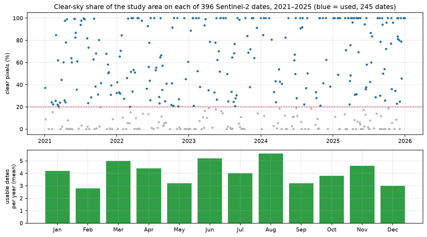
- Read the small SCL band first, drop mostly cloudy dates, then compute NDVI only where it is needed. Here 245 of 396 dates had at least 20% clear pixels, and 67% of the remaining pixel-dates were clear.
- Since processing baseline 04.00 (January 2022), Sentinel-2 L2A digital numbers include a +1000 offset. Forgetting to remove it biases NDVI low across most of the archive.
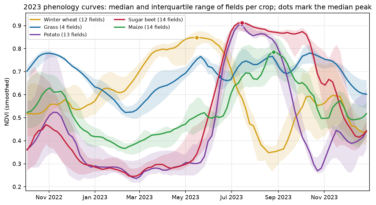
- Smoothed per-field curves separate the crops clearly: in 2023 winter wheat peaked on 16 May, potato and sugar beet on 15 July and maize on 26 August. Sugar beet stayed green until about 28 October, five weeks after potato.
Before you start
- Comfortable with NumPy, pandas and the basics of xarray (the Sentinel-2 Lake Mead tutorial introduces STAC searches and Cloud Optimised GeoTIFFs)
- Python 3.10+ with odc-stac, dask, xarray, pystac-client, planetary-computer, rasterio, geopandas, scipy, matplotlib and imageio
- An internet connection: imagery is streamed from the Microsoft Planetary Computer and needs no account or API key
Short answer: to build an NDVI time series in Python, search the Sentinel-2 L2A archive with pystac-client, then pass the items to odc.stac.load(..., chunks={"time": 1}) to get a lazy, dask-backed xarray datacube with dimensions time × y × x. Mask cloud and shadow with the SCL band (keep classes 4–7), remove the +1000 offset from scenes processed with baseline 04.00 or later, and compute NDVI = (B08 − B04) / (B08 + B04). Then use xarray to aggregate: ndvi.resample(time="1MS").median() for monthly composites, a zonal mean per field for field curves, and a Savitzky–Golay filter to smooth them before reading off phenology dates.
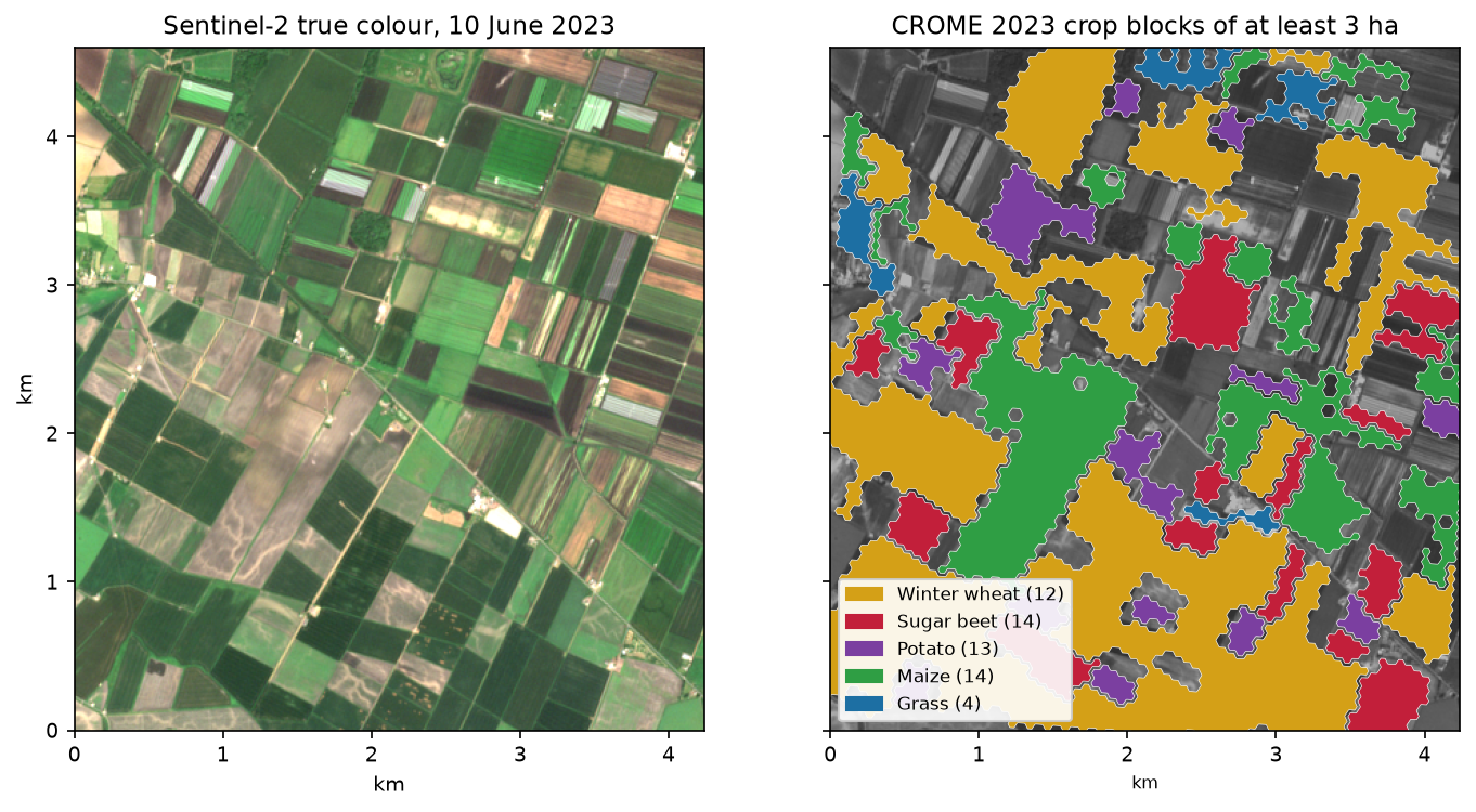
This tutorial follows 57 fields in Methwold Fen, Norfolk, an area of deep, flat Fenland soils in East Anglia that grows winter wheat, sugar beet, potatoes and maize, through five growing seasons (2021–2025). The field boundaries and 2023 crop labels come from the Rural Payments Agency’s Crop Map of England (CROME).
You will learn how to:
- download crop labels for an area from the CROME 2023 web service and turn them into field polygons;
- search every Sentinel-2 L2A scene of one tile for five years with STAC;
- load them as a lazy datacube with odc-stac and dask, and see how much would be read;
- build an SCL cloud mask and keep only usable dates;
- compute NDVI, handling the processing-baseline offset;
- make monthly median composites and small-multiple maps;
- extract a per-field NDVI time series quickly with
np.bincount; - smooth the curves with a Savitzky–Golay filter and estimate green-up, peak and senescence for each crop.
All outputs below are real results from ndvi_time_series.py, run on 17 October 2026 with Python 3.12, odc-stac 0.5.3, xarray 2026.9.0 and dask 2026.8.0.
Why use odc-stac for a Sentinel-2 time series?
A five-year time series of one Sentinel-2 tile is hundreds of scenes, each with a dozen bands stored as separate Cloud Optimised GeoTIFFs. You could open each file with rasterio and stack the arrays yourself, as in our Lake Mead tutorial, but odc-stac does the hard parts for you:
- it reprojects and resamples every item onto one common pixel grid, so scenes from different orbits and tiles line up;
- it mosaics items from the same day (
groupby="solar_day"); - with
chunks=, it returns dask arrays, so building the cube costs almost nothing and only the pixels you actually compute are read, in parallel; - the result is a normal xarray Dataset, so
resample,groupby,whereandmedianwork along the time axis.
stackstac is a popular alternative with a similar idea. The code below would need only small changes to use it.
Step 1: field boundaries and crop labels from CROME
CROME classifies England into hexagons of about 0.4 ha each year, using Sentinel-1 and Sentinel-2 imagery and a machine-learning model trained on field inspections. The 2023 map is published as an ArcGIS feature service. The script downloads the hexagons inside the bounding box in pages of 2000, caches them in a GeoPackage, and then dissolves touching hexagons of the same crop into blocks:
BBOX = (0.40, 52.50, 0.46, 52.54)          # Methwold Fen, Norfolk (lon/lat): about 4 x 4.5 km of Fenland fieldsCRS = "EPSG:32631"                          # UTM zone 31N, the native grid of Sentinel-2 tile 31UCUCROME = ("https://services-eu1.arcgis.com/KB6uNVj5ZcJr7jUP/ArcGIS/rest/services/"         "Crop_Map_of_England_2023/FeatureServer/0/query")CROPS = {"AC66": "Winter wheat", "AC03": "Sugar beet", "AC44": "Potato", "AC17": "Maize", "PG01": "Grass"}MIN_FIELD_HA = 3
while True:   # the service returns at most 2000 hexagons per request: page through them    r = requests.get(CROME, timeout=180, params={        "where": "1=1", "geometry": geom, "geometryType": "esriGeometryEnvelope", "inSR": 4326,        "spatialRel": "esriSpatialRelIntersects", "outFields": "LUCODE,PROB,CROMEID", "outSR": 4326,        "orderByFields": "OBJECTID", "resultOffset": offset, "resultRecordCount": 2000, "f": "geojson"})    page = r.json()    parts.append(gpd.GeoDataFrame.from_features(page["features"], crs=4326))    if len(page["features"]) < 2000:        break    offset += 2000
blocks = hexes[hexes["LUCODE"].isin(CROPS)].dissolve("LUCODE").explode(index_parts=False).reset_index()blocks["crop"] = blocks["LUCODE"].map(CROPS)blocks["geometry"] = blocks.buffer(-10) # shrink 10 m so edge pixels (hedges, tracks) drop outblocks = blocks[~blocks.is_empty].explode(index_parts=False)blocks["area_ha"] = blocks.area / 1e4blocks = blocks[blocks["area_ha"] >= MIN_FIELD_HA]4859 hexagons of 0.42 ha; median classification probability 0.61LUCODEAC66 Winter wheat 1750AC17 Maize 897AC03 Sugar beet 542AC44 Potato 387PG01 Grass 286FA01 229AC01 121AC67 117WO12 106LG20 104median probability by crop: {'Sugar beet': 0.68, 'Maize': 0.37, 'Potato': 0.74, 'Winter wheat': 0.95, 'Grass': 0.26}
=== crop blocks (fields) used for time series === count sum mediancropGrass 4 38.5 10.8Maize 14 236.2 5.7Potato 13 85.5 4.7Sugar beet 14 148.4 7.5Winter wheat 12 637.2 23.6That leaves 57 blocks of at least 3 ha. Note the PROB column: CROME is itself a model output, and its confidence varies a lot by crop. It is very sure about winter wheat (median 0.95) but much less sure about maize (0.37) and grass (0.26), so treat those labels with care.
Step 2: search five years of Sentinel-2 with STAC
The Microsoft Planetary Computer hosts the full Sentinel-2 L2A archive and its STAC API needs no key; planetary_computer.sign_inplace adds a short-lived token to each asset URL. Filtering on s2:mgrs_tile keeps one tile, so every scene has the same footprint. A few dates exist twice, an original and a reprocessed version, so the script keeps the newest processing baseline:
catalog = pystac_client.Client.open("https://planetarycomputer.microsoft.com/api/stac/v1", modifier=planetary_computer.sign_inplace)search = catalog.search(collections=["sentinel-2-l2a"], bbox=BBOX, datetime="2021-01-01/2025-12-31", query={"eo:cloud_cover": {"lt": 80}, "s2:mgrs_tile": {"eq": "31UCU"}})items = list(search.items())best = {} # a few dates exist twice (original and reprocessed): keep the newest processing baselinefor it in items: key = it.datetime.date() if key not in best or it.properties["s2:processing_baseline"] > best[key].properties["s2:processing_baseline"]: best[key] = ititems = sorted(best.values(), key=lambda i: i.datetime)396 Sentinel-2 L2A scenes of tile 31UCU with < 80% cloud, 03 Jan 2021 to 31 Dec 2025{2021: 75, 2022: 81, 2023: 73, 2024: 63, 2025: 104}The tile-level eo:cloud_cover filter is loose on purpose. It describes the whole 110 km tile, not our 4 km area, so a scene that is 70% cloudy overall can still be clear over the fields. The real cloud filtering happens per pixel in Step 4. The jump in 2025 is mostly Sentinel-2C, which began routine operations in January 2025 while Sentinel-2A continued to take some images.
Step 3: load a lazy datacube with odc-stac
This is the core of the tutorial. odc.stac.load builds the datacube from the STAC items:
odc.stac.configure_rio(cloud_defaults=True) # sensible GDAL settings for reading COGs over HTTPds = odc.stac.load( items, bands=["B02", "B03", "B04", "B08", "SCL"], bbox=BBOX, crs=CRS, resolution=10, chunks={"time": 1, "x": 1024, "y": 1024}, # one chunk per scene and band: nothing is read yet groupby="solar_day", dtype="uint16", nodata=0,)ds = ds.assign_coords(time=ds.time.dt.floor("D")) # one scene per day: keep just the dateprint(ds)print(f"{ds.nbytes / 1e9:.2f} GB if loaded in full, in {ds['B04'].data.npartitions} chunks per band")<xarray.Dataset> Size: 772MBDimensions: (y: 460, x: 424, time: 396)Coordinates: * y (y) float64 4kB 5.824e+06 5.824e+06 ... 5.82e+06 5.82e+06 * x (x) float64 3kB 3.235e+05 3.235e+05 ... 3.277e+05 3.277e+05 * time (time) datetime64[us] 3kB 2021-01-03 2021-01-06 ... 2025-12-31 spatial_ref int32 4B 32631Data variables: B02 (time, y, x) uint16 154MB dask.array<chunksize=(1, 460, 424), meta=np.ndarray> B03 (time, y, x) uint16 154MB dask.array<chunksize=(1, 460, 424), meta=np.ndarray> B04 (time, y, x) uint16 154MB dask.array<chunksize=(1, 460, 424), meta=np.ndarray> B08 (time, y, x) uint16 154MB dask.array<chunksize=(1, 460, 424), meta=np.ndarray> SCL (time, y, x) uint16 154MB dask.array<chunksize=(1, 460, 424), meta=np.ndarray>0.77 GB if loaded in full, in 396 chunks per bandThe call returns almost immediately because no pixels have been read: each band is a dask array of 396 chunks, one per date, and each chunk knows which windowed reads of which COGs it needs. A few points about the arguments:
crsandresolutionfix the output grid. Using the tile’s own UTM zone at 10 m avoids resampling the 10 m bands. The 20 m SCL band is upsampled with nearest neighbour.chunks={"time": 1, ...}gives one chunk per scene. That suits per-date operations such as cloud masking. For per-pixel operations along time, such as a median over a whole season, rechunk later to{"time": -1}.dtype="uint16", nodata=0keep the raw digital numbers. Converting to float32 would double the memory before you need it.groupby="solar_day"mosaics items acquired on the same day, which matters when your area spans two tiles or two adjacent orbit segments.
Step 4: SCL cloud masking
The scene classification layer labels each pixel. The script keeps vegetation (4), bare soil (5), water (6) and unclassified (7), and treats cloud shadow (3), medium and high cloud (8, 9) and cirrus (10) as cloudy. SCL usually misses the soft edges of clouds, so the cloudy pixels are grown by three pixels (30 m). Reading only the SCL band first is cheap, and it tells us which dates are worth reading in full:
KEEP_SCL = [4, 5, 6, 7] # vegetation, bare soil, water, unclassifiedMIN_CLEAR = 0.2 # skip scenes where less than 20% of the area is cleardask.config.set(scheduler="threads", num_workers=16)scl = ds["SCL"].compute()cloudy = np.isin(scl.values, [3, 8, 9, 10]) # cloud shadow, cloud (medium, high), cirrusgrown = ndimage.binary_dilation(cloudy, iterations=3, axes=(1, 2)) # grow by 30 m: edges are often missedclear = scl.isin(KEEP_SCL) & ~xr.DataArray(grown, coords=scl.coords, dims=scl.dims)clear_frac = clear.mean(("y", "x")).to_series()read SCL for 396 dates in 4 s
=== clear-sky fraction per scene ===245 of 396 dates have at least 20% clear pixelsshare of usable scenes by month (%): {1: 66, 2: 58, 3: 61, 4: 59, 5: 50, 6: 63, 7: 59, 8: 68, 9: 55, 10: 61, 11: 74, 12: 65}axes=(1, 2) dilates in space only, not across dates. It needs SciPy 1.15 or later.
Step 5: compute NDVI, with the processing-baseline offset
Sentinel-2 L2A digital numbers are reflectance × 10,000. From processing baseline 04.00, introduced on 25 January 2022, ESA adds an offset of +1000 so that negative reflectances can be stored. On the Planetary Computer, most older scenes have not been reprocessed, so a five-year cube mixes both conventions. The script builds a per-date offset from the items’ s2:processing_baseline property:
baseline = pd.Series({pd.Timestamp(i.datetime.date()): float(i.properties["s2:processing_baseline"]) for i in items})offset = xr.DataArray(np.where(baseline.reindex(ds.time.dt.floor("D").values).values >= 4.0, 1000, 0),                      dims="time", coords={"time": ds.time})

def ndvi_of(sub: xr.Dataset) -> xr.DataArray:    """NDVI from L2A digital numbers. Baseline 04.00+ (from 25 Jan 2022) stores reflectance x 10000 + 1000."""    off = offset.sel(time=sub.time).astype("float32")    red = (sub["B04"].astype("float32") - off) / 10000    nir = (sub["B08"].astype("float32") - off) / 10000    return ((nir - red) / (nir + red)).where((sub["B04"] > 0) & (sub["B08"] > 0))

keep_times = clear_frac.index[clear_frac >= MIN_CLEAR]lazy = ndvi_of(ds.sel(time=keep_times)).where(clear.sel(time=keep_times))ndvi = lazy.compute().rename("ndvi")lazy NDVI: float32, {'time': 245, 'y': 460, 'x': 424}, 245 chunkscomputed NDVI for 245 dates in 14 s
=== NDVI cube ==={'time': 245, 'y': 460, 'x': 424}, 67.4% of pixel-dates clearNDVI percentiles 5/50/95: [0.189 0.559 0.898]ds.sel(time=keep_times) drops the cloudy dates before anything is computed, so dask reads the red and NIR bands for 245 dates instead of 396. The whole step took 14 seconds. The script caches the result in a NetCDF file, so later runs skip the download.
Step 6: monthly median composites
With the time series in xarray, monthly composites are one line. A median ignores NaN (cloud) and is robust to a single bad observation, such as cloud shadow that SCL missed:
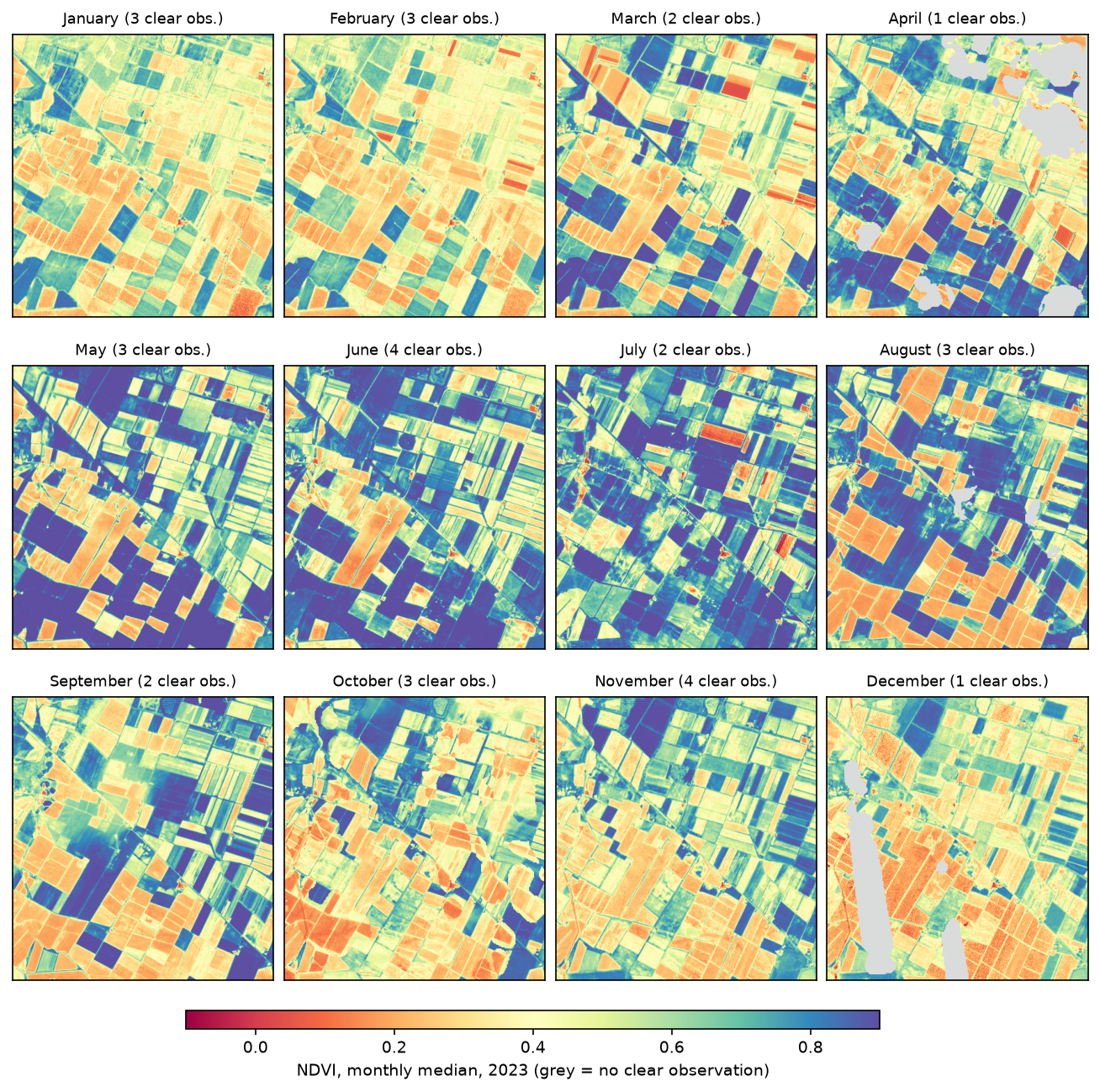
monthly = ndvi.resample(time="1MS").median()n_obs = ndvi.notnull().resample(time="1MS").sum()cover = monthly.notnull().mean(("y", "x"))monthly.astype("float32").to_netcdf(OUT / "ndvi_monthly_median_2021_2025.nc")60 months; 47 have NDVI for at least 95% of pixels, 1 have none Jan Feb Mar Apr May Jun Jul Aug Sep Oct Nov Decmedian NDVI 0.44 0.42 0.49 0.54 0.69 0.73 0.74 0.63 0.55 0.43 0.51 0.41clear obs/pixel 3 3 2 1 3 4 2 3 2 3 4 1cover % 100 100 100 87 100 100 100 99 100 100 100 91Small multiples, one map per month, are the clearest way to show a datacube on a static page. The script also writes the same twelve frames as an animated GIF (output/ndvi_2023.gif) with imageio, which is handy for slides and social media.
Step 7: a per-field NDVI time series
To get one value per field and date, rasterise the field polygons onto the same grid as the cube, then sum the NDVI of each field’s pixels with np.bincount. That is much faster than a zonal-statistics loop over polygons, and it lets you require that most of a field is clear before using its value:
gbox = ds.odc.geobox # the cube's grid: shape, CRS and affine transformlabels = rasterio.features.rasterize(zip(blocks.geometry, blocks["field_id"]), out_shape=gbox.shape, transform=gbox.affine, fill=0, dtype="int32")n_pix = np.bincount(labels.ravel(), minlength=len(blocks) + 1)MIN_FIELD_CLEAR = 0.8 # a field counts as observed on a date only if 80% of its pixels are clearrows = []for t in range(ndvi.sizes["time"]): a = ndvi.isel(time=t).values.ravel() ok = np.isfinite(a) s = np.bincount(labels.ravel()[ok], weights=a[ok], minlength=len(blocks) + 1) c = np.bincount(labels.ravel()[ok], minlength=len(blocks) + 1) frac = c / np.maximum(n_pix, 1) for f in np.nonzero(frac[1:] >= MIN_FIELD_CLEAR)[0] + 1: rows.append((pd.Timestamp(ndvi.time.values[t]).normalize(), f, s[f] / c[f], frac[f]))ts = pd.DataFrame(rows, columns=["date", "field_id", "ndvi", "clear_frac"])8159 field-dates for 57 fields; median 144 clear observations per field over five yearsdate 2021 2022 2023 2024 2025cropGrass 93 104 105 91 196Maize 300 348 364 317 664Potato 299 336 360 303 632Sugar beet 280 359 359 322 666Winter wheat 261 274 314 250 562import odc.geo.xr registers the .odc accessor on xarray objects, which gives the cube’s geobox. The result is a tidy table, also written to field_ndvi_timeseries.csv, with about 29 clear observations per field per year.
Step 8: smooth the curves and estimate phenology
Raw field means are still noisy: thin cloud and shadow that SCL missed pull NDVI down, almost never up. A standard fix (Chen et al., 2004) is an upper-envelope Savitzky–Golay filter: interpolate onto a regular 5-day grid, fit the filter, replace observations far below the curve with the fitted value, and repeat:
STEP = "5D"                      # resample to a regular 5-day grid before filteringWINDOW, ORDER = 9, 2             # 9 x 5 days = 45-day window, quadratic fit

def smooth(series: pd.Series, start: str = "2021-01-01", end: str = "2025-12-31") -> pd.Series:    """Upper-envelope Savitzky-Golay smoothing (after Chen et al., 2004) on a regular 5-day grid."""    grid = pd.date_range(start, end, freq=STEP)    s = series.groupby(level=0).mean()    for _ in range(3):           # observations far below the curve are probably cloud or shadow: pull them up        filled = s.reindex(s.index.union(grid)).interpolate("time", limit_direction="both").reindex(grid)        fit = pd.Series(savgol_filter(filled.values, WINDOW, ORDER), index=grid)        on_fit = fit.reindex(s.index, method="nearest")        s = s.where(s >= on_fit - 0.05, on_fit)    return fit.clip(-0.2, 1)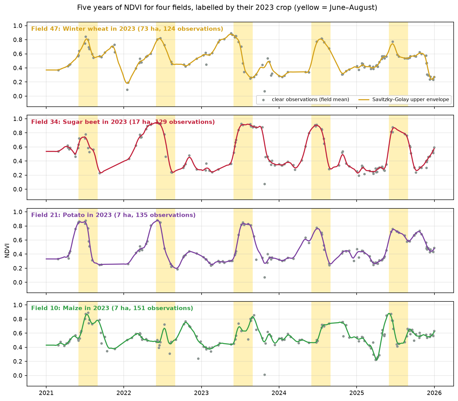
For phenology, the script finds the 2023 peak and the dates where the smoothed curve crosses 50% of the seasonal amplitude on the way up (green-up) and down (senescence or harvest). Thresholds of 20–50% are all common; 50% is the most robust to noise.
def phenology(curve: pd.Series, year: int) -> dict:    """Green-up, peak and senescence dates where the curve crosses 50% of the seasonal amplitude."""    c = curve[f"{year - 1}-10-01":f"{year}-12-31"]    peak = c[f"{year}-03-01":f"{year}-10-31"].idxmax()    lo_before, lo_after = c[:peak].min(), c[peak:].min()    up = c[:peak][c[:peak] < lo_before + 0.5 * (c[peak] - lo_before)]    down = c[peak:][c[peak:] < lo_after + 0.5 * (c[peak] - lo_after)]    return {"green_up": up.index[-1] if len(up) else pd.NaT, "peak": peak, "peak_ndvi": c[peak],            "senescence": down.index[0] if len(down) else pd.NaT, "amplitude": c[peak] - min(lo_before, lo_after)}

curves = {f: smooth(g.set_index("date")["ndvi"]) for f, g in ts.groupby("field_id") if len(g) >= 40}pheno = pd.DataFrame([dict(field_id=f, **phenology(c, 2023)) for f, c in curves.items()]) fields green_up peak peak_ndvi senescencecropWinter wheat 12 25 Feb 16 May 0.87 20 JulGrass 4 01 Apr 15 Jun 0.80 16 AugPotato 13 10 Jun 15 Jul 0.91 23 SepSugar beet 14 05 Jun 15 Jul 0.91 28 OctMaize 14 25 Jun 26 Aug 0.83 15 OctThe results match the Fenland crop calendar well:
- Winter wheat, sown in autumn, is already green over winter, greens up strongly in late February and peaks in mid-May. NDVI falls as the crop ripens and is harvested in late July and August.
- Potato and sugar beet are planted in spring, cover the ground in June and both peak in mid-July at an NDVI of 0.91. Potato haulm is destroyed before lifting, so potato NDVI falls in September; sugar beet stays green until it is lifted, here from late October.
- Maize is sown in May, greens up last (late June) and peaks in late August.
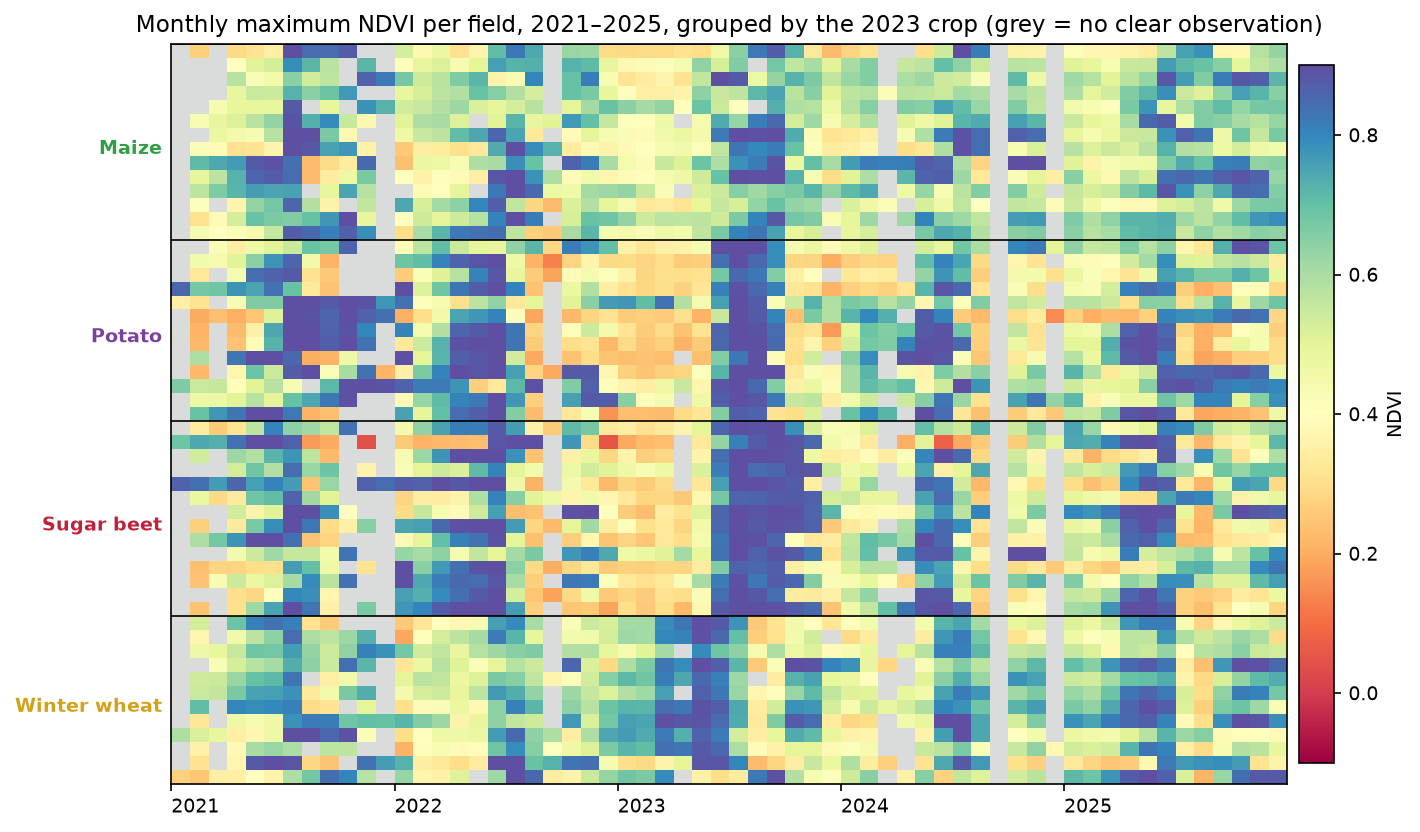
Finally, a heatmap of the monthly maximum NDVI of every field shows crop rotation. Each row is a field and each column a month. In 2023 almost every potato and sugar beet row is dark blue from late June to September, and the winter wheat rows peak earlier, in spring. In the other years the same rows are far less consistent, because each field carried a different crop.
Pitfalls and limitations
- The labels are a model too. CROME is produced by a machine-learning classifier, and its own confidence is low for maize (median 0.37) and grass (0.26) here. Some “maize” blocks may be another spring crop. For research, use field-inspection data or the farm’s own records.
- Blocks are not exactly fields. Dissolving hexagons merges neighbouring fields with the same crop, and the hexagon edges cut across field boundaries. The 10 m inward buffer helps, but some blocks still include tracks and margins. Real field boundaries (for example from the Rural Payments Agency’s land parcels, where you have access) are better.
- One year of labels. The crop labels apply to 2023 only. The 2021, 2022, 2024 and 2025 curves belong to whatever was grown then.
- SCL misses some cloud. Thin cirrus, haze and shadow from small clouds get through; the upper-envelope filter and the 80% field-clear rule reduce, but do not remove, the effect. Low outliers in the field plots are mostly missed cloud. For better masks, try s2cloudless or the OmniCloudMask model.
- Gaps change the dates. Phenology dates are only as good as the observations around them. A cloudy fortnight at green-up can shift the 50% crossing by a week or more, and the 45-day filter window smooths very quick changes such as harvest.
- One tile. The script uses only tile 31UCU. Neighbouring tiles and orbits add more dates, but they need care with the processing baseline and different viewing angles.
- NDVI saturates. Above an NDVI of about 0.85, dense canopies look alike. For biomass or yield work, try the red-edge index NDRE or EVI.
Frequently asked questions
How do I create an NDVI time series in Python?
Search Sentinel-2 L2A scenes with pystac-client, load them into an xarray datacube with odc.stac.load (or stackstac), mask cloud with the SCL band, compute NDVI from bands B08 and B04 after removing the +1000 offset in newer scenes, and reduce over space: a zonal mean per field or a median over an area. Then smooth with a Savitzky–Golay filter. The full, runnable script is linked above.
What is the difference between odc-stac and stackstac?
Both turn STAC items into a dask-backed xarray object. odc-stac returns an xarray.Dataset with one variable per band, groups items by day, and supports per-band resampling and data types. stackstac returns one DataArray with a band dimension and is a little more minimal. Both are maintained and fast; odc-stac is used by Digital Earth Australia and Digital Earth Africa.
How do I mask clouds in Sentinel-2 with Python?
For L2A data, the simplest method is the SCL band: keep vegetation, bare soil, water and unclassified (classes 4–7) and mask cloud shadow, cloud and cirrus (3, 8, 9 and 10). Grow the cloud mask by a few pixels, because SCL often misses cloud edges. For better accuracy, use a machine-learning mask such as s2cloudless (the S2_CLOUD_PROBABILITY product) or OmniCloudMask.
Why do my Sentinel-2 NDVI values drop in 2022?
Probably because of the processing-baseline offset. Since baseline 04.00 (25 January 2022), L2A digital numbers have 1000 added. If you divide by 10,000 without first subtracting 1000, red and NIR are both 0.1 too high, which lowers NDVI. Read s2:processing_baseline from each STAC item and subtract the offset where it is 04.00 or later, as in Step 5.
How many clear Sentinel-2 images will I get per year?
It depends on the climate. In this East Anglian example, 245 of 396 scenes (62%) over five years had at least 20% of the area clear, about 49 dates per year, and the median field had 144 clear observations over five years. Western Britain and Ireland get fewer. Sentinel-2C, which began routine operations in 2025, increased the number of scenes noticeably here.
Can I use Landsat as well?
Yes. Harmonised Landsat Sentinel-2 (HLS) data provides Landsat 8 and 9 and Sentinel-2 on a common 30 m grid with matching bands, which roughly doubles the number of observations. On the Planetary Computer, landsat-c2-l2 can be loaded with the same odc.stac.load call, but you need to apply its own scale and offset and its QA cloud mask.
Next steps
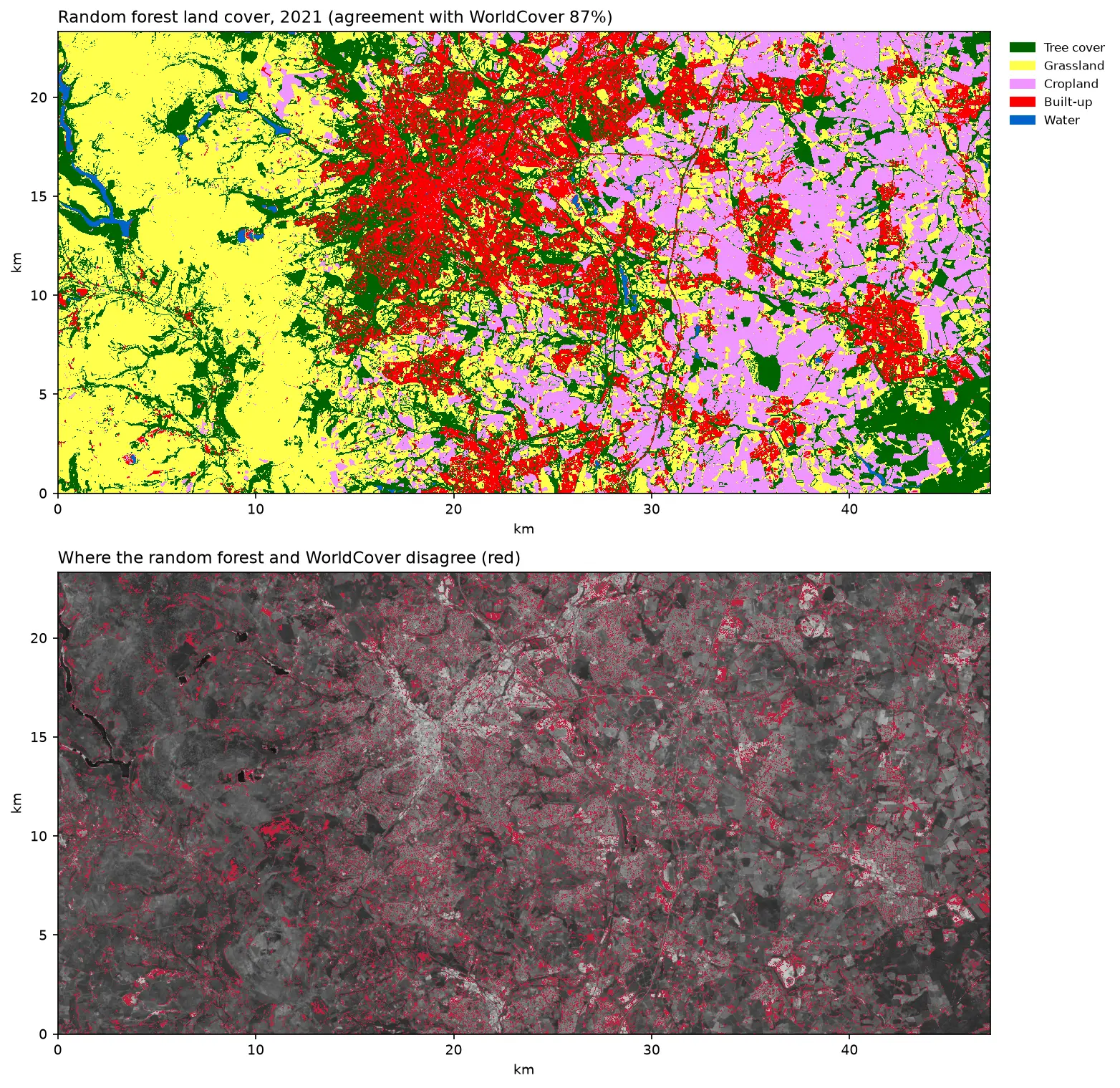
- Use the phenology curves as features to classify crops, as in our companion tutorial land cover classification with a random forest.
- Swap the 4 km area for a whole farm or county and run the same code on a
dask.distributedcluster. - Learn the STAC basics on a single date in Measuring Lake Mead’s shrinking shoreline with Sentinel-2 and STAC, or apply time-series thinking to water in reservoir water quality with Sentinel-2.
- When cloud blocks optical data, track crops and flooding with radar instead: Sentinel-1 SAR flood mapping in Python.
- New to vector data in Python? Start with GeoPandas: getting started.
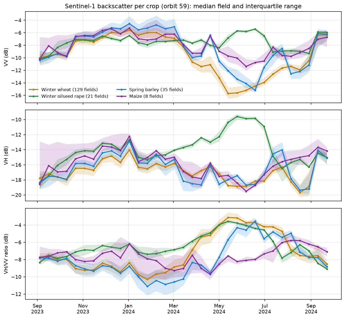
- When cloud leaves gaps in the NDVI record, follow wheat and oilseed rape with radar instead in Sentinel-1 crop monitoring in Python.
Data and licences
- Sentinel-2 L2A: contains modified Copernicus Sentinel data 2021–2025, processed by ESA. Accessed as Cloud Optimised GeoTIFFs from the Microsoft Planetary Computer on 17 October 2026.
- Crop Map of England (CROME) 2023: © Rural Payments Agency, licensed under the Open Government Licence v3.0. Accessed through the CROME 2023 feature service on 17 October 2026.
- References: Chen, J. et al. (2004), “A simple method for reconstructing a high-quality NDVI time-series data set based on the Savitzky–Golay filter”, Remote Sensing of Environment 91(3–4); Rouse, J. W. et al. (1974), “Monitoring vegetation systems in the Great Plains with ERTS”, NASA SP-351.
- Code:
ndvi_time_series.py, tested with Python 3.12.0, odc-stac 0.5.3, xarray 2026.9.0, dask 2026.8.0, pystac-client 0.9.0, planetary-computer 1.0.0 and scipy 1.18.1.
Key terms
- NDVI
- Normalised Difference Vegetation Index, (NIR − red) / (NIR + red), using Sentinel-2 bands B08 and B04. Dense green vegetation scores about 0.8–0.9, bare soil 0.1–0.3 and water below 0.
- odc-stac
- A Python library from the Open Data Cube project that loads STAC items into an xarray Dataset on a common pixel grid, optionally as lazy dask arrays.
- Datacube
- A stack of co-registered images with dimensions such as time, y and x, so that a pixel's whole history can be read as one array.
- SCL
- The Sentinel-2 L2A scene classification layer: a 20 m band that labels each pixel as cloud, cloud shadow, vegetation, bare soil, water, snow and so on.
- Savitzky–Golay filter
- A smoothing filter that fits a low-order polynomial in a moving window. It keeps the height and timing of peaks better than a moving average.
- Phenology
- The timing of the stages in a plant's life cycle, such as green-up, peak growth and senescence, here estimated from the NDVI curve.
Data for this tutorial
- Microsoft Planetary Computer · Sentinel-2 L2A as Cloud Optimised GeoTIFFs via STAC
- UK data sources · Crop Map of England (CROME) 2023, Rural Payments Agency
Licences and formats for each source are listed in the GIS data sources catalogue.