Land cover classification in Python: a Sentinel-2 random forest with scikit-learn

Short answer: for supervised land cover classification in Python, build a cloud-free feature stack (for example seasonal Sentinel-2 median composites of the bands plus NDVI and other indices), collect labelled pixels for each class, train a scikit-learn RandomForestClassifier, and assess it on test data that is spatially separate from the training data, using a confusion matrix and per-class F1 scores. Then call predict on every pixel and save the result as a GeoTIFF. Assess accuracy with blocked cross-validation (GroupKFold on spatial blocks), not a random split, because neighbouring pixels are nearly identical.

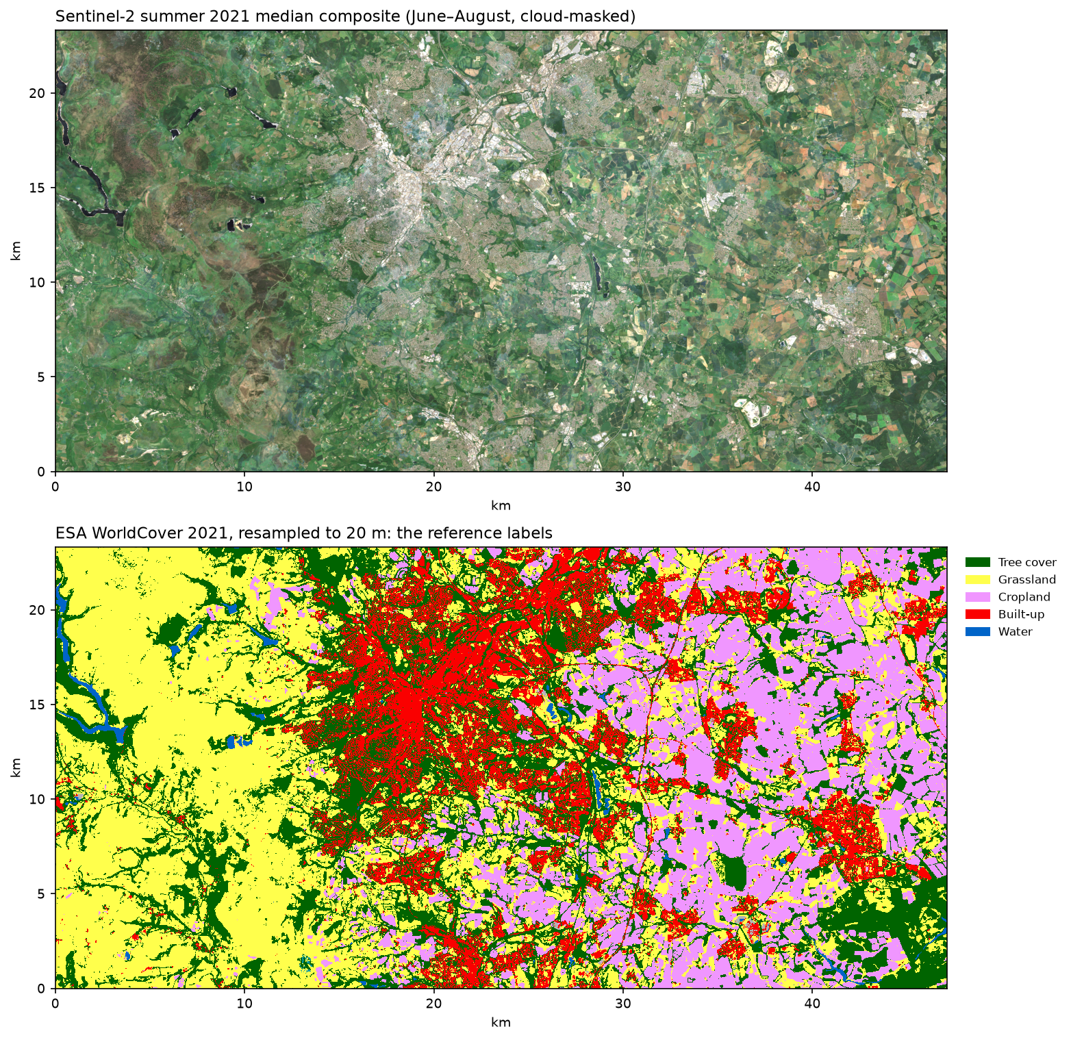
This tutorial classifies a 47 × 23 km area of Sheffield and the Peak District in northern England, which runs from heather and grass moorland with reservoirs in the west, through the city, to arable farmland and woodland in the east. It uses Sentinel-2 imagery for 2021 and training labels sampled from ESA WorldCover 2021.

You will learn how to:

1. search a growing season of Sentinel-2 with STAC and build spring, summer and autumn median composites with odc-stac and dask;
2. turn them into a feature stack of bands plus NDVI, MNDWI, NDBI and NDRE;
3. load ESA WorldCover onto the same grid and draw a stratified random sample of training pixels;
4. train a random forest and test it on held-out 2 km spatial blocks;
5. compare random and spatially blocked cross-validation;
6. read a confusion matrix and per-class F1 scores;
7. rank features with permutation importance;
8. predict a full land cover map and see how it compares with the reference.

All outputs below are real results from land_cover_random_forest.py, run on 17 October 2026 with Python 3.12, scikit-learn 1.9.1, odc-stac 0.5.3 and xarray 2026.9.0.

Step 1: search one growing season of Sentinel-2

A single image only shows one moment. Crops are bare in spring and green in summer, while grass is green almost all year, so several dates make classes much easier to separate. WorldCover 2021 describes 2021, so the script uses Sentinel-2 scenes from March to October of that year. The area spans two Sentinel-2 tiles (30UWE and 30UXE), so duplicates are removed per date and tile:

BBOX = (-1.75, 53.25, -1.05, 53.45)        # Peak District moors, Sheffield and the farmland to the east
CRS, RES = "EPSG:32630", 20                # UTM zone 30N at 20 m: the native grid of the red-edge and SWIR bands
YEAR = 2021                                # match the year of the ESA WorldCover map used for the labels
SEASONS = {"spring": [3, 4, 5], "summer": [6, 7, 8], "autumn": [9, 10]}
BANDS = ["B02", "B03", "B04", "B05", "B06", "B07", "B08", "B8A", "B11", "B12"]

catalog = pystac_client.Client.open(STAC_URL, modifier=planetary_computer.sign_inplace)
items = catalog.search(collections=["sentinel-2-l2a"], bbox=BBOX, datetime=f"{YEAR}-03-01/{YEAR}-10-31",
                       query={"eo:cloud_cover": {"lt": 60}}).item_collection()
best = {}   # keep the newest processing baseline when a date and tile exist twice
for it in items:
    key = (it.datetime.date(), it.properties["s2:mgrs_tile"])
    if key not in best or it.properties["s2:processing_baseline"] > best[key].properties["s2:processing_baseline"]:
        best[key] = it
items = sorted(best.values(), key=lambda i: i.datetime)

68 Sentinel-2 L2A items (tiles ['30UWE', '30UXE']) with < 60% cloud, 07 Mar to 11 Oct 2021

The classification works at 20 m, the native resolution of the red-edge (B05–B07, B8A) and shortwave infrared (B11, B12) bands. The 10 m bands are averaged to 20 m. That quarters the number of pixels compared with 10 m and suits WorldCover, which is resampled to the same grid in Step 4.

Step 2: seasonal median composites with odc-stac

odc.stac.load builds a lazy datacube from the 68 items, mosaicking the two tiles on each date (groupby="solar_day"). The cloud mask uses the scene classification (SCL) band, as in the NDVI time series tutorial: keep classes 4–7, and grow cloud and shadow by two pixels (40 m). Then, for each season, the script takes the median of the clear observations:

ds = odc.stac.load(items, bands=BANDS + ["SCL"], bbox=BBOX, crs=CRS, resolution=RES,
                   chunks={"time": 1, "x": 2048, "y": 2048}, groupby="solar_day", dtype="uint16", nodata=0,
                   resampling={"*": "average", "SCL": "nearest"})
ds = ds.assign_coords(time=ds.time.dt.floor("D"))
gbox = ds.odc.geobox

scl = ds["SCL"].compute()
cloudy = np.isin(scl.values, [3, 8, 9, 10])                          # shadow, cloud (medium, high), cirrus
grown = ndimage.binary_dilation(cloudy, iterations=2, axes=(1, 2))   # grow by 40 m
clear = scl.isin([4, 5, 6, 7]) & ~xr.DataArray(grown, coords=scl.coords, dims=scl.dims)
frac = clear.mean(("y", "x")).to_series()
layers = {}
for season, months in SEASONS.items():
    times = frac.index[(frac >= 0.1) & frac.index.month.isin(months)]
    sub = ds[BANDS].sel(time=times)
    refl = ((sub.astype("float32") - offset.sel(time=times)) / 10000).where(clear.sel(time=times))
    med = refl.chunk({"time": -1, "y": 512, "x": 512}).median("time").compute()
    for b in BANDS:
        layers[f"{season}_{b}"] = med[b]
comp = xr.Dataset(layers)

lazy cube: {'y': 1166, 'x': 2356, 'time': 42}, 2.5 GB if loaded in full
dropped 0 dates whose tiles mix processing baselines before and after 04.00
SCL read in 3 s; 36 of 42 dates are at least 10% clear
spring  18 dates; pixels with no clear view: 0.31%
summer   9 dates; pixels with no clear view: 0.69%
autumn   9 dates; pixels with no clear view: 0.78%
composites built in 47 s

Two details matter:

• Rechunk before the median. The cube is loaded with one chunk per date, which is right for reading. A median along time needs every date for a pixel in one chunk, so .chunk({"time": -1, "y": 512, "x": 512}) swaps to small spatial tiles holding the full time series.
• The processing-baseline offset. Scenes processed with baseline 04.00 or later store reflectance × 10,000 + 1000. The offset array holds 0 or 1000 per date, built from each item’s s2:processing_baseline. The script drops any date whose two tiles use different conventions, because they are mosaicked together; in 2021 there were none.

Even in a wet English summer, the medians leave less than 1% of pixels with no clear view in any season.

Step 3: features: bands plus spectral indices

Each season contributes its ten bands and four normalised-difference indices. A random forest could in principle learn these ratios from the bands, but giving them directly makes the trees shallower and the model more robust:

def nd(a, b):
    return (a - b) / (a + b)


features = {}
for s in SEASONS:
    for b in BANDS:
        features[f"{s}_{b}"] = comp[f"{s}_{b}"]
    features[f"{s}_NDVI"] = nd(comp[f"{s}_B08"], comp[f"{s}_B04"])      # vegetation
    features[f"{s}_MNDWI"] = nd(comp[f"{s}_B03"], comp[f"{s}_B11"])     # open water
    features[f"{s}_NDBI"] = nd(comp[f"{s}_B11"], comp[f"{s}_B08"])      # built-up and bare surfaces
    features[f"{s}_NDRE"] = nd(comp[f"{s}_B8A"], comp[f"{s}_B05"])      # red-edge chlorophyll
FEATURES = list(features)
X_all = np.stack([features[f].values.astype("float32") for f in FEATURES], axis=-1)   # (y, x, feature)
H, W, F = X_all.shape

1166 x 2356 pixels of 20 m, 42 features (3 seasons x (10 bands + 4 indices))
pixels with at least one missing feature: 1.56%

The result is an ordinary NumPy array of shape (rows, columns, features), which is what scikit-learn needs. At 2.7 million pixels × 42 features × 4 bytes it is about 460 MB, so for a much larger area, process it in tiles.

Step 4: training labels from ESA WorldCover

ESA WorldCover is also on the Planetary Computer. Passing the composite’s geobox to odc.stac.load puts it on exactly the same 20 m grid. resampling="mode" takes the most common 10 m class in each 20 m pixel, which is the right choice for categorical data:

wc_items = catalog.search(collections=["esa-worldcover"], bbox=BBOX,
                          query={"esa_worldcover:product_version": {"eq": "2.0.0"}}).item_collection()
wc = odc.stac.load(wc_items, bands=["map"], geobox=gbox, resampling="mode").squeeze("time")["map"].values
share = pd.Series(wc.ravel()).value_counts(normalize=True).sort_index()
MIN_SHARE = 0.005                         # drop classes covering less than 0.5% of the area
USE = [c for c in CLASSES if share.get(c, 0) >= MIN_SHARE]

10 Tree cover            27.21
20 Shrubland              0.00
30 Grassland             36.99
40 Cropland              20.87
50 Built-up              14.05
60 Bare / sparse          0.14
80 Water                  0.72
90 Herbaceous wetland     0.02
classes used: ['Tree cover', 'Grassland', 'Cropland', 'Built-up', 'Water']; dropped: ['Shrubland', 'Bare / sparse', 'Herbaceous wetland']

Version 2.0.0 is the 2021 map. Three classes cover less than 0.5% of the area and are dropped, because a few hundred pixels, possibly misclassified, cannot train a class reliably. Pixels of those classes are still predicted as one of the five classes used.

Step 5: a stratified random sample of pure pixels

With five classes of very different sizes (water is 0.7%, grassland 37%), a simple random sample would contain almost no water. A stratified random sample draws the same number from each class. The script also keeps only “pure” pixels whose 3 × 3 neighbourhood is all the same class, which removes mixed pixels on boundaries and many of the reference map’s edge errors:

N_PER_CLASS = 2000
BLOCK = 2000                              # 2 km x 2 km spatial blocks for the train/test split
rng = np.random.default_rng(SEED)
valid = ~np.isnan(X_all).any(-1)
rows, cols, ys = [], [], []
for c in USE:
    # Keep pixels whose 3 x 3 neighbourhood is all the same class: fewer mixed pixels and edge errors.
    pure = ndimage.binary_erosion(wc == c, structure=np.ones((3, 3))) & valid
    r, cc = np.nonzero(pure)
    pick = rng.choice(len(r), size=min(N_PER_CLASS, len(r)), replace=False)
    rows.append(r[pick]); cols.append(cc[pick]); ys.append(np.full(len(pick), c))
rows, cols, y = np.concatenate(rows), np.concatenate(cols), np.concatenate(ys)
X = X_all[rows, cols]
block_px = BLOCK // RES
block_id = (rows // block_px) * (W // block_px + 1) + cols // block_px

Tree cover    2000
Grassland     2000
Cropland      2000
Built-up      2000
Water         2000
10000 samples in 288 blocks of 2 km

Each sample also records which 2 km × 2 km block it falls in. Those blocks drive the train/test split in the next step.

Step 6: train a random forest and test on spatial blocks

Pixels close together look alike. If you split samples randomly, most test pixels have a training pixel a few tens of metres away, and the model can “recognise” them rather than generalise. That makes accuracy look better than it will be on new areas. The fix is to split by space: put every block into one of five folds, and hold out fold 0 (about 20% of blocks) entirely for testing:

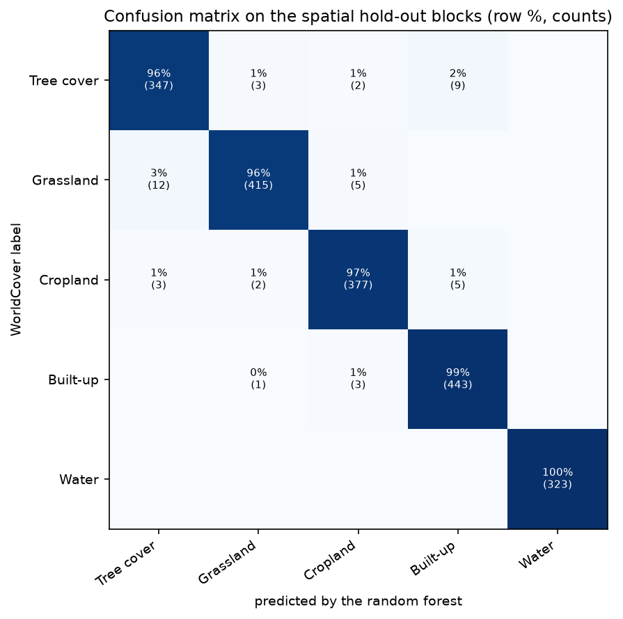
blocks = np.unique(block_id)
fold_of_block = dict(zip(blocks, rng.permutation(len(blocks)) % 5))
fold = np.array([fold_of_block[b] for b in block_id])
test = fold == 0                                            # one fifth of the blocks are held out entirely
rf = RandomForestClassifier(n_estimators=300, max_features="sqrt", min_samples_leaf=1, n_jobs=-1,
                            random_state=SEED, oob_score=True)
rf.fit(X[~test], y[~test])
pred = rf.predict(X[test])
print(classification_report(y[test], pred, labels=USE, target_names=names, digits=3))

trained on 8050 samples in 0.6 s; tested on 1950 samples
overall accuracy 0.977 | macro F1 0.977 | out-of-bag accuracy 0.972
              precision    recall  f1-score   support

  Tree cover      0.959     0.961     0.960       361
   Grassland      0.986     0.961     0.973       432
    Cropland      0.974     0.974     0.974       387
    Built-up      0.969     0.991     0.980       447
       Water      1.000     1.000     1.000       323

    accuracy                          0.977      1950
   macro avg      0.978     0.977     0.977      1950
weighted avg      0.977     0.977     0.977      1950

area-weighted accuracy (class recall weighted by WorldCover area share): 0.968

Random forests need little tuning. 300 trees and max_features="sqrt" (about 6 of the 42 features tried at each split) are standard defaults; more trees rarely help much. The out-of-bag score (97.2%) is a free estimate from the samples each tree did not see, but it uses random samples, so it has the same spatial leakage problem as a random split.

Because the sample is balanced, overall accuracy treats each class equally. The area-weighted accuracy (96.8%) weights each class’s recall by its share of the map, which is closer to what a map user experiences. In remote sensing terms, precision is user’s accuracy and recall is producer’s accuracy.

Random vs spatially blocked cross-validation

One hold-out fold is a small test. Five-fold cross-validation uses every sample once for testing. The script runs it twice, with KFold (random) and with GroupKFold using the spatial folds as groups:

for name, splitter, groups in [("random", KFold(5, shuffle=True, random_state=SEED), None),
                               ("spatial blocks", GroupKFold(5), fold)]:
    p = cross_val_predict(RandomForestClassifier(n_estimators=300, n_jobs=-1, random_state=SEED), X, y,
                          cv=splitter, groups=groups)

random          accuracy 0.973 | macro F1 0.973 | Tree 0.96 Grassland 0.96 Cropland 0.97 Built-up 0.98 Water 1.00
spatial blocks  accuracy 0.971 | macro F1 0.971 | Tree 0.96 Grassland 0.96 Cropland 0.97 Built-up 0.97 Water 1.00
random CV overstates accuracy by 0.2 percentage points

Here the gap is tiny. That is an honest result, and it has a reason: 10,000 samples spread over about 2.7 million pixels are, on average, hundreds of metres apart, so few test pixels have a near-twin in the training set. The gap grows when samples are dense, for example when every pixel inside hand-drawn training polygons is used, which is the usual way of working in desktop GIS. Then random splits put neighbouring pixels from the same polygon on both sides and can overstate accuracy by 10 points or more. Blocked cross-validation costs nothing extra, so use it by default.

Step 7: how good is the whole map?

The tests above all use pure pixels, which are the easy ones. The real question is how the model does on every pixel, including field edges, hedgerows, gardens and mixed pixels. Since WorldCover covers the whole area, the script can compare every pixel:

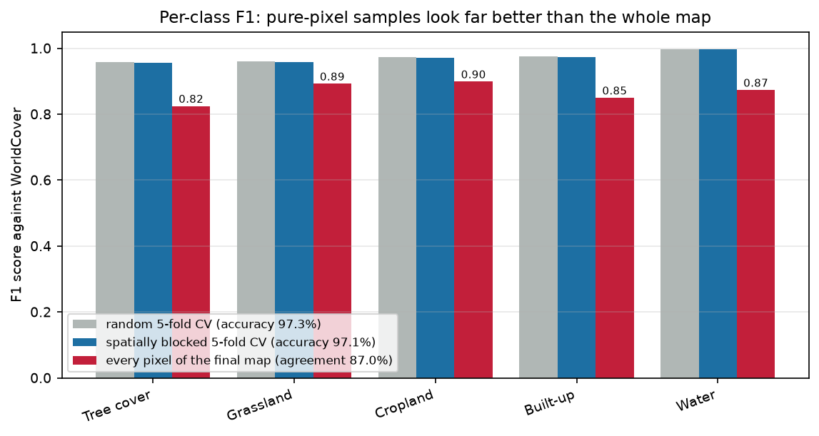
predicted 2,747,096 pixels in 6 s
agreement with WorldCover over the classes used: 87.0%; median top-class probability 0.96
per-class F1 against WorldCover over every pixel: Tree 0.82 Grassland 0.89 Cropland 0.90 Built-up 0.85 Water 0.87

That is a drop of about 10 points, and it is the most important lesson of this tutorial. A test set drawn the same way as the training set inherits its biases. Excluding edge pixels made both training and testing cleaner, but the map still has to label those edges. A proper accuracy assessment uses an independent, probability-based sample of the whole map, labelled by people, as described by Olofsson et al. (2014).

Step 8: feature importance

Impurity-based importance (rf.feature_importances_) is quick but biased towards features with many distinct values, and it spreads credit across correlated features. Permutation importance on the held-out test blocks is more honest: shuffle one feature and see how much macro F1 drops:

pi = permutation_importance(rf, X[test], y[test], n_repeats=5, random_state=SEED, n_jobs=-1, scoring="f1_macro")
imp = pd.DataFrame({"permutation": pi.importances_mean, "perm_sd": pi.importances_std,
                    "impurity": rf.feature_importances_}, index=FEATURES).sort_values("permutation", ascending=False)

              permutation  perm_sd  impurity
spring_MNDWI       0.0121   0.0007    0.0423
autumn_NDRE        0.0039   0.0016    0.0661
spring_B11         0.0034   0.0013    0.0536
spring_B8A         0.0030   0.0016    0.0624
spring_B08         0.0024   0.0013    0.0436
summer_NDRE        0.0020   0.0010    0.0513
impurity importance by season: {'autumn': 0.292, 'spring': 0.39, 'summer': 0.318}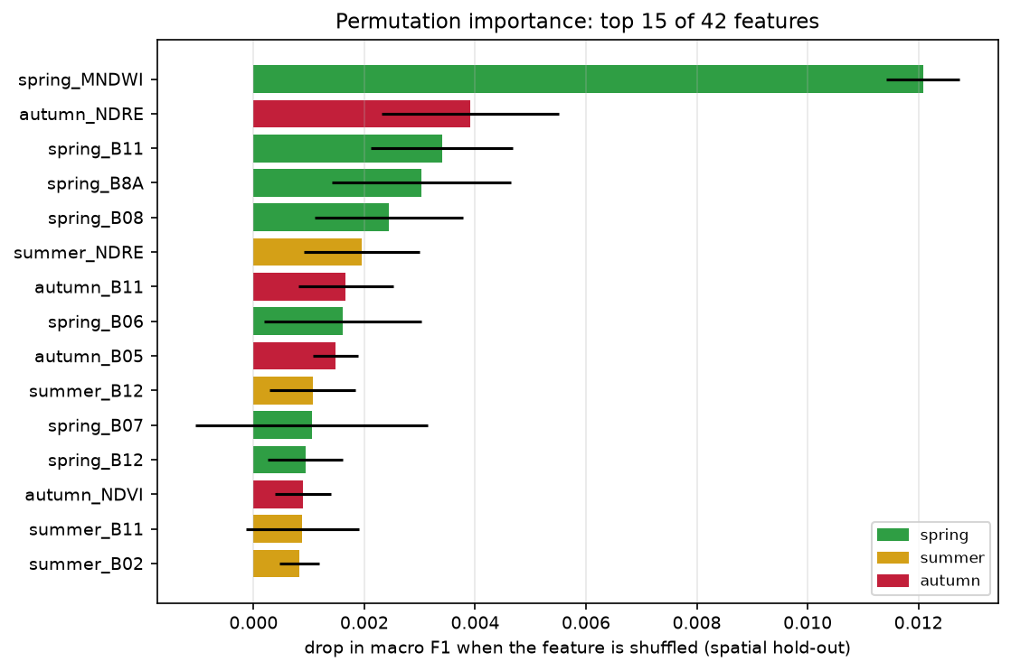

The drops are all small, because the 42 features are highly correlated: shuffle one, and the forest uses a near-copy from another season. Treat the ranking as a hint rather than a measurement. Still, it makes sense: in spring, arable fields are bare or sparsely covered, so shortwave infrared (B11) and the water index separate them from grass. The red-edge index NDRE separates crops, grass and trees by chlorophyll content, and spring features as a group carry the most weight (0.39 of impurity importance). If you need fewer features, drop correlated ones and check that blocked cross-validation does not get worse.

Predicting the full map

The final model is trained on all 10,000 samples and applied to every pixel in chunks of 200,000 to limit memory. Since scikit-learn 1.4, random forests handle NaN in features, so the 1.6% of pixels with a missing season still get a prediction. The result is written as a GeoTIFF with the WorldCover colour table, ready for QGIS:

final = RandomForestClassifier(n_estimators=300, max_features="sqrt", n_jobs=-1, random_state=SEED).fit(X, y)
flat = X_all.reshape(-1, F)
pred_map = np.zeros(H * W, dtype="uint8")
for i in range(0, H * W, 200_000):                          # predict in chunks to keep memory low
    proba = final.predict_proba(flat[i:i + 200_000])        # scikit-learn >= 1.4 forests accept missing values
    pred_map[i:i + 200_000] = final.classes_[proba.argmax(1)]
pred_map = pred_map.reshape(H, W)
with rasterio.open(OUT / "land_cover_rf_2021.tif", "w", driver="GTiff", height=H, width=W, count=1, dtype="uint8",
                   crs=CRS, transform=gbox.affine, compress="deflate", nodata=0) as dst:
    dst.write(pred_map, 1)

            WorldCover_ha  random_forest_ha
Tree cover          29897             26388
Grassland           40651             40093
Cropland            22928             25171
Built-up            15437             17527
Water                 796               705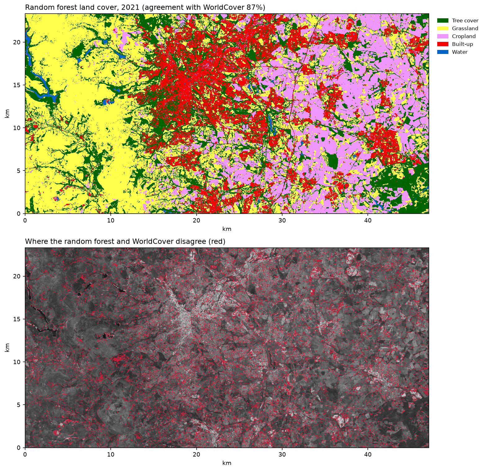

The map looks very like WorldCover, which is what it was trained to do. It has less tree cover (−12%) and more built-up land (+14%) and cropland (+10%). Many of the differences are in the suburbs, where a 20 m pixel of houses and gardens with trees is genuinely mixed, so neither map is clearly right. To learn which is closer to the truth you would need independent reference data.

Pitfalls and limitations

• The labels are a map, not the truth. WorldCover’s global overall accuracy is about 77%, and its errors become training data. It also maps most heather moorland in the Peak District as grassland, so this model cannot learn a heath class. Hand-labelled points or polygons are better, and essential for any published map.
• Pure-pixel tests are optimistic. As Step 7 shows, accuracy on samples drawn away from edges (97.7%) is much higher than agreement over every pixel (87.0%). Report accuracy from an independent sample of the whole map.
• Blocked cross-validation is not a guarantee. 2 km blocks reduce leakage between nearby pixels, but every block is still in the same landscape. The model may do worse in, say, East Anglia or Scotland.
• Rare classes were dropped. Shrubland, bare ground and wetland together cover about 0.2% of this area. Their pixels are forced into one of the five classes.
• Balanced training changes the priors. Training with 2000 samples per class tells the model that water is as common as grassland. That favours small classes in ambiguous pixels. You can rebalance, or use class_weight, if area estimates matter.
• Clouds and composites. Median composites hide most cloud, but SCL misses some haze and shadow, and pixels with few clear dates are noisier.
• One year. The model is trained for 2021 imagery; applying it to another year needs new composites and, ideally, a check against new reference data.

Frequently asked questions

How do I do supervised classification in Python?

Build a feature array where each pixel is a row (for example by stacking Sentinel-2 bands and indices with NumPy or xarray), collect labelled pixels, fit a scikit-learn classifier such as RandomForestClassifier, check accuracy on spatially separate test data, then call predict on every pixel and reshape the result back into an image. Rasterio writes it as a GeoTIFF. This tutorial’s script does every step on real data.

Why use a random forest for Sentinel-2 classification?

Random forests are accurate, fast, need almost no tuning, cope with correlated features and different value ranges without scaling, give class probabilities and handle missing values. Gradient boosting (LightGBM, XGBoost) is often slightly more accurate but needs more tuning. Deep learning (for example U-Nets) can use spatial context but needs far more labelled data.

How many training samples do I need?

Hundreds to a few thousand per class is typical for a random forest. More important than the number is that samples cover the variety within each class (for example, different crops and different kinds of woodland) and the whole area. Thousands of samples from a few polygons are worth less than a few hundred spread widely.

What is spatial cross-validation and why does it matter?

It groups samples by location, for example into 2 km blocks, and holds out whole blocks. A random split puts neighbouring, nearly identical pixels in both training and test sets, which can make accuracy look much better than it really is. In scikit-learn, use GroupKFold with block IDs as groups. In R, CAST and blockCV do the same.

Can I use ESA WorldCover or Dynamic World as training data?

For learning and prototyping, yes, as here. For a real product, it means copying another map’s errors. If you use one, keep only pixels where two maps agree (for example WorldCover and Esri’s IO-LULC), use pure pixels away from edges, and check the result against independent, hand-labelled points.

How would I do this in Google Earth Engine?

The workflow maps across directly: filter COPERNICUS/S2_SR_HARMONIZED and mask clouds, make seasonal median() composites, add indices, stratifiedSample the ESA/WorldCover/v200 map, train ee.Classifier.smileRandomForest(300), classify the image, and use errorMatrix for accuracy. Earth Engine runs the computation on Google’s servers, which is convenient for very large areas. We use open STAC data here because Earth Engine needs a Google account and a registered Cloud project, and because the Python version lets you use any scikit-learn model and validation method, including blocked cross-validation, which Earth Engine does not provide out of the box.

Next steps

• Build crop-specific features from a time series instead of seasonal medians, as in NDVI time series in Python with odc-stac.
• Add terrain: elevation and slope help separate moorland, woodland and farmland. See raster terrain analysis with rasterio.
• Add Sentinel-1 radar features, which see through cloud and are sensitive to structure, as in Sentinel-1 SAR flood mapping in Python.
• Turn the map into polygons and summarise land cover by area with fast vector geoprocessing, or share it on an interactive web map with Folium.
• Start with the STAC basics in Measuring Lake Mead’s shrinking shoreline with Sentinel-2 and STAC.
• Segment individual objects such as buildings and fields, rather than classifying pixels, with Segment Anything on satellite and aerial imagery.

Data and licences

• Sentinel-2 L2A: contains modified Copernicus Sentinel data 2021, processed by ESA. Accessed as Cloud Optimised GeoTIFFs from the Microsoft Planetary Computer on 17 October 2026.
• ESA WorldCover 2021 (v200): © ESA WorldCover project 2021 / Contains modified Copernicus Sentinel data (2021) processed by the ESA WorldCover consortium. Licensed under CC BY 4.0. Accessed from the Planetary Computer on 17 October 2026. Zanaga, D. et al. (2022), ESA WorldCover 10 m 2021 v200, doi:10.5281/zenodo.7254221.
• References: Breiman, L. (2001), “Random forests”, Machine Learning 45; Olofsson, P. et al. (2014), “Good practices for estimating area and assessing accuracy of land change”, Remote Sensing of Environment 148; Roberts, D. R. et al. (2017), “Cross-validation strategies for data with temporal, spatial, hierarchical, or phylogenetic structure”, Ecography 40(8).
• Code: land_cover_random_forest.py, tested with Python 3.12.0, scikit-learn 1.9.1, odc-stac 0.5.3, xarray 2026.9.0, dask 2026.8.0 and pystac-client 0.9.0.