Burn severity mapping with Sentinel-2 and dNBR in Python (Saddleworth Moor 2018)

Short answer: to map burn severity with dNBR in Python, choose a clear Sentinel-2 L2A image from just before the fire and one from just after it. Calculate the Normalised Burn Ratio for both, NBR = (B8A − B12) / (B8A + B12), and mask cloud, shadow and water with the SCL band. Then subtract: dNBR = NBR_pre − NBR_post. Remove the small offset found on unburned ground nearby and classify dNBR with the USGS thresholds (0.10, 0.27, 0.44 and 0.66 for low, moderate-low, moderate-high and high). Multiply each class’s pixel count by the pixel area to get hectares. For the 2018 Saddleworth Moor fire this gives a 1,078 ha burn perimeter, of which 519 ha is high severity.

On 24 June 2018, during the long, dry summer of that year, a fire broke out on Saddleworth Moor above Greenfield and Stalybridge, on the north-west edge of the Peak District. It flared up again on 26 June and strong winds spread it quickly over the next few days. Homes in nearby Carrbrook were evacuated, soldiers were brought in to help the fire service, and crews were still damping down hotspots well into July. Sentinel-2 imaged the moor every few days throughout, with almost no cloud, so it is an ideal case study for burn severity mapping. It is also just north of the reservoirs in our Peak District water quality tutorial.

You will learn how to:

1. find the pre- and post-fire Sentinel-2 L2A scenes with a STAC search and read them on their native 20 m grid;
2. convert digital numbers to reflectance, including the processing baseline offset, and mask cloud, shadow and water with SCL;
3. do the NBR calculation and compute dNBR with an offset from unburned ground;
4. classify dNBR into the USGS severity classes, measure the burned area in hectares and export a burn perimeter;
5. map the fire’s progression from successive images;
6. compute RdNBR and see when it disagrees with dNBR;
7. follow the scar’s recovery from 2017 to 2025.

All outputs below are real results from burn_severity_dnbr.py, run on 17 October 2026 with Python 3.12, pystac-client 0.9.0, planetary-computer 1.0.0, rasterio 1.5.2 and numpy 2.5.4.

Why the Normalised Burn Ratio works

Healthy plants reflect a lot of near-infrared light (NIR), because of the structure of their leaves, and absorb shortwave infrared (SWIR) light, because of the water they contain. Fire reverses both: it removes the leaves and leaves charcoal, ash and dry, bare soil or peat, which are dark in the NIR and relatively bright in the SWIR. The Normalised Burn Ratio combines the two bands that change most:

NBR = (NIR − SWIR2) / (NIR + SWIR2)

For Sentinel-2 that is (B8A − B12) / (B8A + B12). B8A (865 nm) is the narrow NIR band; it is 20 m like B12 (2190 nm), so the two match pixel for pixel. Some scripts use the 10 m B8 instead, which also works. For Landsat 8 and 9 the same formula uses bands 5 and 7.

One image is not enough. Moorland, bare peat, rock and towns all have a low NBR without ever burning. So we compare the same place before and after the fire. This difference is dNBR: positive where NBR fell (vegetation lost), close to zero where nothing changed, and negative where vegetation grew.

Step 1: find the pre- and post-fire Sentinel-2 scenes

We define a 10.5 × 8.0 km study area around Saddleworth Moor, Buckton Moor and Dovestone Reservoir. We snap it to multiples of 20 m in UTM zone 30N so that the pixels line up exactly with Sentinel-2’s own 20 m grid, which avoids resampling. Then we search the Microsoft Planetary Computer for every image of tile 30UWE from June to August 2018:

STAC_URL = "https://planetarycomputer.microsoft.com/api/stac/v1"
AOI = (-2.06, 53.475, -1.90, 53.545)   # lon/lat: Saddleworth Moor, Buckton Moor and Dovestone, Peak District
CRS = "EPSG:32630"                     # UTM zone 30N, the native grid of Sentinel-2 tile 30UWE
TILE = "30UWE"
RES = 20                               # B8A and B12 are both 20 m bands
PRE, POST = "2018-06-24", "2018-07-14"
PROGRESSION = ["2018-06-26", "2018-06-29", "2018-07-04", "2018-07-14"]

to_utm = Transformer.from_crs("EPSG:4326", CRS, always_xy=True)
xs, ys = to_utm.transform([AOI[0], AOI[2]], [AOI[1], AOI[3]])
x0, y0 = np.floor(min(xs) / RES) * RES, np.floor(min(ys) / RES) * RES   # snap to the native 20 m grid
x1, y1 = np.ceil(max(xs) / RES) * RES, np.ceil(max(ys) / RES) * RES
WIDTH, HEIGHT = int((x1 - x0) / RES), int((y1 - y0) / RES)
TRANSFORM = from_origin(x0, y1, RES, RES)
BOUNDS = (x0, y0, x1, y1)
HA_PER_PX = RES * RES / 10_000          # one 20 m pixel = 0.04 ha

catalog = pystac_client.Client.open(STAC_URL)
search = catalog.search(collections=["sentinel-2-l2a"], bbox=AOI, datetime="2018-06-01/2018-08-31",
                        query={"s2:mgrs_tile": {"eq": TILE}, "eo:cloud_cover": {"lt": 50}})
summer = {it.datetime.strftime("%Y-%m-%d"): it for it in search.items()}

grid: 526 x 398 pixels of 20 m (10.5 x 8.0 km), EPSG:32630
11 scenes of tile 30UWE with < 50% cloud, June to August 2018
2018-06-24  Sentinel-2B  scene cloud  10.5%  baseline 02.12  sun zenith 31.4
2018-06-26  Sentinel-2A  scene cloud   6.7%  baseline 02.12  sun zenith 32.0
2018-06-29  Sentinel-2A  scene cloud   0.3%  baseline 02.12  sun zenith 31.6
2018-07-04  Sentinel-2B  scene cloud   3.0%  baseline 02.12  sun zenith 32.0
2018-07-14  Sentinel-2B  scene cloud  11.0%  baseline 02.12  sun zenith 33.3

The choice of dates matters more than anything else in a dNBR map:

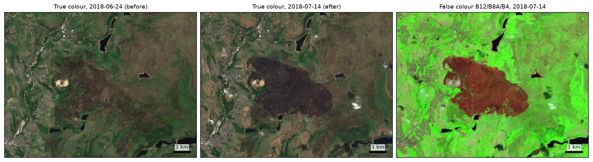
• Pre-fire: 24 June 2018. Sentinel-2 passes over at about 11:00 UTC, and this image shows no burn scar, so it shows the moor just before it burned. In an early test we used a clear image from May instead. The moor dried and browned so much during the drought between May and late June that large unburned areas showed up as “low severity”. Keep the gap between the two dates as short as you can.
• Post-fire: 14 July 2018. By then the fire had burned out over almost the whole area, and the image is clear. An image taken months later would show regrowth and would understate severity. The USGS uses both an initial assessment, soon after the fire, and an extended assessment, at the start of the next growing season. With forests the extended assessment is often better; on moorland that greens up quickly, the initial one is more useful.

Step 2: convert to reflectance and mask cloud, shadow and water

Each band is read as a window of a Cloud Optimised GeoTIFF, without downloading the full 110 × 110 km tile. Two details are easy to miss:

• The processing baseline. Since 25 January 2022 (baseline 04.00), Sentinel-2 L2A digital numbers include an offset of +1000. Reflectance is (DN − 1000) / 10000 for newer scenes and DN / 10000 for older ones. The 2018 scenes are baseline 02.12, but the recovery series in Step 7 mixes both, so the function checks.
• The SCL band. The scene classification layer labels cloud, cloud shadow, cirrus, snow, water and saturated pixels. We remove them all and buffer the cloud mask by three pixels (60 m), because cloud edges and thin shadows are rarely classified perfectly. We remove water too, because the NBR of water changes randomly from date to date.

BAD_SCL = [0, 1, 3, 8, 9, 10, 11]   # no data, saturated, cloud shadow, cloud medium/high, cirrus, snow
WATER_SCL = 6


def to_reflectance(dn: np.ndarray, item) -> np.ndarray:
    """L2A digital numbers to surface reflectance. Baseline 04.00+ (from 25 Jan 2022) adds a -1000 offset."""
    offset = -1000 if float(item.properties["s2:processing_baseline"]) >= 4.0 else 0
    return np.where(dn > 0, (dn.astype("float32") + offset) / 10_000, np.nan)


def nbr(nir: np.ndarray, swir2: np.ndarray) -> np.ndarray:
    """Normalised Burn Ratio = (NIR - SWIR2) / (NIR + SWIR2), with B8A and B12 for Sentinel-2."""
    with np.errstate(divide="ignore", invalid="ignore"):
        return (nir - swir2) / (nir + swir2)


def load_scene(date: str, bands=("B8A", "B12", "B04", "B03", "B02")) -> dict:
    """Reflectance, NBR and a clear-land mask for one date, cached as .npz."""
    f = CACHE / f"s2_{date}_{len(bands)}.npz"
    if not f.exists():
        item = summer[date]
        arr = {b: to_reflectance(read_band(item, b), item) for b in bands}
        arr["SCL"] = read_band(item, "SCL")
        np.savez_compressed(f, **arr)
    s = dict(np.load(f))
    cloud = ndimage.binary_dilation(np.isin(s["SCL"], BAD_SCL[1:]), iterations=3)   # 60 m buffer round cloud
    s["clear"] = ~cloud & (s["SCL"] != 0) & (s["SCL"] != WATER_SCL) & np.isfinite(s["B12"])
    s["NBR"] = nbr(s["B8A"], s["B12"])
    return s


pre, post = load_scene(PRE), load_scene(POST)
valid = pre["clear"] & post["clear"]

read_band (in the full script) signs the asset URL with planetary_computer.sign, reads a window with rasterio and retries if the connection drops. Ten-metre bands are averaged to 20 m and SCL is resampled with nearest neighbour.

pre  SCL: vegetation 92.5%, not vegetated 5.2%, water 1.2%, cloud/shadow/cirrus 0.1%
post SCL: vegetation 77.6%, not vegetated 16.5%, water 1.2%, cloud/shadow/cirrus 0.5%
pixels clear on both dates: 203,975 of 209,348 (97.4%)

The jump in “not vegetated” from 5.2% to 16.5% is the fire scar itself. Only 2.6% of the area is lost to cloud, shadow, the 60 m buffer and water.

Step 3: NBR calculation and dNBR

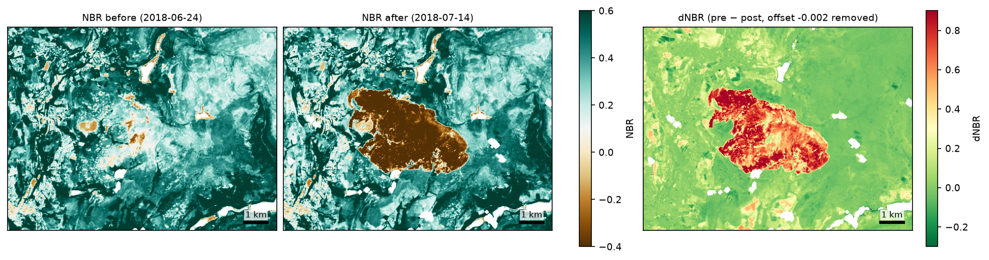
With the two scenes masked, the NBR calculation is already done inside load_scene, and dNBR is a single subtraction:

dnbr_raw = np.where(valid, pre["NBR"] - post["NBR"], np.nan)

# A first, generous burn mask finds the scar so that we can measure the unburned background around it.
seed = ndimage.binary_opening(np.nan_to_num(dnbr_raw) > 0.27, iterations=1)
lab, n = ndimage.label(seed)
sizes = ndimage.sum(seed, lab, index=np.arange(1, n + 1))
scar = np.isin(lab, 1 + np.flatnonzero(sizes * HA_PER_PX >= 50))          # patches of at least 50 ha
near = ndimage.binary_dilation(scar, iterations=50)                       # within 1 km of the scar
ring = near & ~ndimage.binary_dilation(scar, iterations=15) & valid       # 300 m to 1 km outside it
OFFSET = float(np.nanmedian(dnbr_raw[ring]))
dnbr = dnbr_raw - OFFSET

The offset corrects for differences between the two dates that have nothing to do with the fire: a change in sun angle, haze, or vegetation drying out. Ideally, unburned ground has a dNBR of zero. We measure it in a ring 300 m to 1 km outside the scar and subtract the median. Key and Benson recommend the same idea; they also scale dNBR by 1000, so a USGS threshold of 270 is 0.27 here.

median NBR: pre-fire 0.414, post-fire 0.364
dNBR 0.5th-99.5th percentile: -0.139 to 0.996
unburned reference ring: 1,025 ha, median dNBR -0.002 -> subtracted as the offset

In this case the offset is tiny, −0.002, because the two images are only 20 days apart and both were taken in a dry, stable spell. With images from different seasons or sensors it can easily be ±0.05 or more, which would move hundreds of hectares between classes.

Step 4: USGS severity classes and burned area in hectares

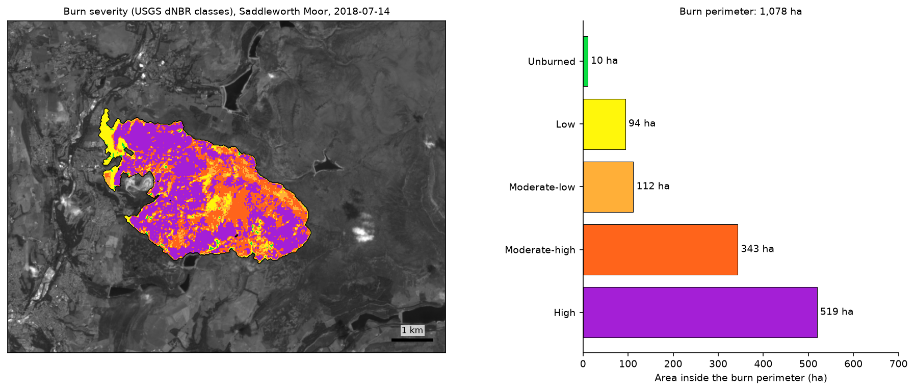
The most widely used thresholds come from Key and Benson (2006), as published by the USGS and the UN-SPIDER knowledge portal. We classify the offset-corrected dNBR, then build a burn perimeter from every pixel of low severity or worse that touches the main scar. A morphological opening removes isolated noisy pixels, and a closing fills small gaps:

CLASSES = [  # Key and Benson (2006) dNBR ranges, as published by USGS and UN-SPIDER
    ("Enhanced regrowth, high", -np.inf, -0.251, "#7a8737"),
    ("Enhanced regrowth, low", -0.251, -0.101, "#acbe4d"),
    ("Unburned", -0.101, 0.099, "#0ae042"),
    ("Low severity", 0.099, 0.269, "#fff70b"),
    ("Moderate-low severity", 0.269, 0.439, "#ffaf38"),
    ("Moderate-high severity", 0.439, 0.659, "#ff641b"),
    ("High severity", 0.659, np.inf, "#a41fd6"),
]
edges = [c[2] for c in CLASSES[:-1]]
cls = np.where(np.isfinite(dnbr), np.digitize(dnbr, edges, right=True), 255).astype("uint8")   # 0..6, 255 = masked

# Burn perimeter: low severity or worse, cleaned, in patches connected to the main scar.
burned = ndimage.binary_opening((cls >= 3) & (cls < 255), iterations=1)
lab, n = ndimage.label(burned)
keep = np.unique(lab[scar & burned])
perimeter = np.isin(lab, keep[keep > 0])
perimeter = ndimage.binary_closing(perimeter, iterations=2) & np.isfinite(dnbr)

rows = []
for k, (name, lo, hi, _) in enumerate(CLASSES):
    rng = f"< {hi:.3f}" if lo == -np.inf else (f">= {lo:.3f}" if hi == np.inf else f"{lo:.3f} to {hi:.3f}")
    rows.append({"class": name, "dNBR range": rng,
                 "whole AOI (ha)": round((cls == k).sum() * HA_PER_PX, 1),
                 "inside perimeter (ha)": round(((cls == k) & perimeter).sum() * HA_PER_PX, 1)})
area = pd.DataFrame(rows)

Each 20 m pixel is 400 m², or 0.04 ha, so the area of a class is simply its pixel count × 0.04. That only works because the grid is in a projected CRS with metre units; never count pixels in latitude and longitude.

                  class       dNBR range  whole AOI (ha)  inside perimeter (ha)  % of burn
Enhanced regrowth, high         < -0.251             4.7                    0.0        NaN
 Enhanced regrowth, low -0.251 to -0.101            91.8                    0.0        NaN
               Unburned  -0.101 to 0.099          5929.9                   10.1        NaN
           Low severity   0.099 to 0.269           989.2                   93.8        8.8
  Moderate-low severity   0.269 to 0.439           237.9                  111.5       10.4
 Moderate-high severity   0.439 to 0.659           386.1                  343.2       32.1
          High severity         >= 0.659           519.5                  519.1       48.6
burn perimeter: 1,078 ha (10.8 km2); moderate-low or worse: 974 ha
whole AOI at low severity or worse: 2,116 ha without the offset, 2,133 ha with it
perimeter polygon: 1,078 ha, 28.9 km of edge

Two numbers deserve a closer look:

• Low severity outside the scar: 895 ha. The whole study area has 989 ha in the low class, but only 94 ha of it is inside the perimeter. The rest is scattered across fields and moorland that never burned. It comes from the drought (grass browned between the two dates) and from farmers cutting hay and silage. This is why you need a perimeter step and should not report “everything with dNBR > 0.1” as burned.
• High severity is almost all inside the scar (519.1 of 519.5 ha). Very high dNBR values are hard to produce any other way.

The script also saves dnbr_2018.tif, a colour-mapped severity_classes_2018.tif and the perimeter as burn_perimeter_2018.gpkg, ready for QGIS.

Step 5: map the fire’s progression

Because Sentinel-2 imaged the moor four times between 26 June and 14 July, we can see when each part of the scar burned. We compare each image with the pre-fire image and record the first date on which each pixel’s dNBR exceeds 0.27 (moderate-low or worse):

first_seen = np.zeros((HEIGHT, WIDTH), dtype="uint8")
prog = []
zone = ndimage.binary_dilation(perimeter, iterations=5)
for k, d in enumerate(PROGRESSION, 1):
    s = load_scene(d, bands=("B8A", "B12"))
    ok = pre["clear"] & s["clear"]
    burnt_now = ok & zone & ((pre["NBR"] - s["NBR"] - OFFSET) > 0.27)
    first_seen[burnt_now & (first_seen == 0)] = k
    prog.append({"date": d, "clear_in_perimeter_%": round(100 * ok[perimeter].mean(), 1),
                 "burnt_ha": int(round(burnt_now.sum() * HA_PER_PX))})

      date  clear_in_perimeter_%  burnt_ha
2018-06-26                  93.5        27
2018-06-29                 100.0       913
2018-07-04                 100.0       956
2018-07-14                 100.0       974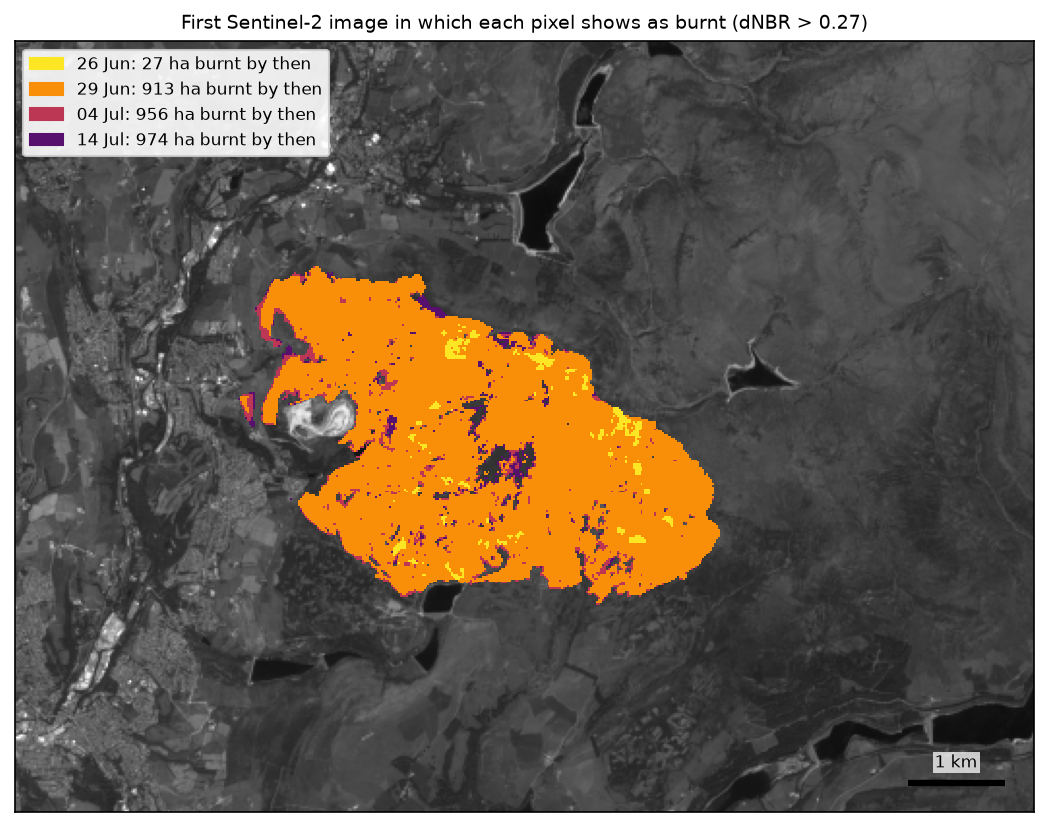

Only 27 ha had burned by the morning of 26 June, but 913 ha had burned by 29 June. That matches the reports of the fire spreading rapidly in strong winds over those days. The 6.5% of the perimeter under cloud on 26 June means the first number is a slight underestimate. A satellite image every two to five days is no substitute for fire-service records, but it is a free and independent way to reconstruct the timeline.

Step 6: RdNBR, the relative version of dNBR

dNBR measures an absolute change, so it depends on how much vegetation was there before. Burning a dense stand of heather from NBR 0.6 to −0.3 gives a dNBR of 0.9. Completely burning a sparse patch of grass and bare peat from NBR 0.1 to −0.2 gives only 0.3, even though nothing was left in either case. Miller and Thode (2007) proposed the relative dNBR to correct for this:

RdNBR = dNBR / √|NBR_pre|

pre_nbr = np.where(valid, pre["NBR"], np.nan)
with np.errstate(divide="ignore", invalid="ignore"):
    rdnbr = dnbr / np.sqrt(np.clip(np.abs(pre_nbr), 0.001, None))   # Miller and Thode (2007), unscaled units
m = perimeter & np.isfinite(rdnbr)
low_pre = m & (pre_nbr < np.percentile(pre_nbr[m], 25))
high_pre = m & (pre_nbr > np.percentile(pre_nbr[m], 75))
RDNBR_EDGES = [0.069, 0.316, 0.641]   # Miller and Thode (2007): 69, 316, 641 on their x1000 scale
rd_cls = np.digitize(rdnbr[m], RDNBR_EDGES)
dn_cls = np.digitize(dnbr[m], [0.1, 0.27, 0.66])

The clip at 0.001 stops the division blowing up where pre-fire NBR is close to zero. Miller and Thode worked with NBR and dNBR multiplied by 1000 and divided by √|NBR_pre / 1000|, so their RdNBR values are 1000 times ours: their thresholds of 69, 316 and 641 are 0.069, 0.316 and 0.641 here. Always check which scaling a set of thresholds assumes.

pre-fire NBR inside the perimeter: median 0.288, 5th-95th pct 0.001 to 0.550
inside perimeter: median dNBR 0.647, median RdNBR 1.340
lowest quarter of pre-fire NBR:  median dNBR 0.510, RdNBR 1.609
highest quarter of pre-fire NBR: median dNBR 0.796, RdNBR 1.133
hectares inside the perimeter by four-class scheme:
  unchanged  RdNBR      3 ha | dNBR     11 ha
  low        RdNBR     61 ha | dNBR     94 ha
  moderate   RdNBR     67 ha | dNBR    456 ha
  high       RdNBR    947 ha | dNBR    518 ha

The two indices tell different stories:

• dNBR says the sparsest quarter of the moor (lowest pre-fire NBR) burned least severely, with a median of 0.510, and the densest quarter most severely, 0.796. That is largely because there was more to lose.
• RdNBR reverses the order: 1.609 for the sparsest quarter and 1.133 for the densest. Relative to what was there, the sparse areas lost the most.
• With the Miller and Thode thresholds, RdNBR puts 947 ha in the high class against 518 ha for dNBR. Those thresholds were calibrated in Sierra Nevada conifer forest, and with a pre-fire NBR as low as 0.29 almost any burn crosses them. They should not be applied to moorland without local field data.

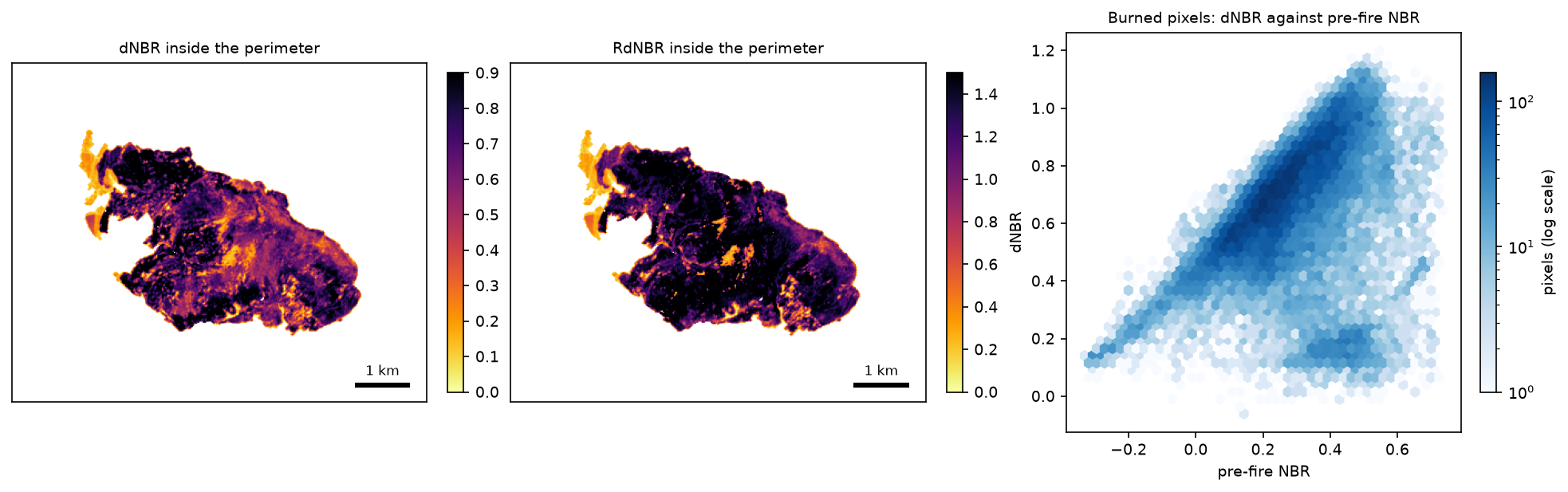
RdNBR is most useful for comparing fires in different vegetation types, or a mosaic of sparse and dense vegetation, as here. For a single fire in a homogeneous landscape, dNBR is simpler and more widely understood. A third variant, RBR (relativised burn ratio, Parks et al., 2014), divides by NBR_pre + 1.001 and avoids the instability near zero.

Step 7: follow the recovery from 2017 to 2025

Finally, we take every May–September image of the area from 2017 to 2025, keep those where at least 80% of both the burned area and an unburned control ring are clear, and record the median NBR of each. Comparing the burned area with the control removes most of the year-to-year variation caused by weather:

def recovery_row(item) -> dict:
    """Median NBR of the burned and control pixels in one scene, if both are at least 80% clear."""
    scl = read_band(item, "SCL", SUB)
    ok = ~np.isin(scl, BAD_SCL + [WATER_SCL])
    row = {"date": item.datetime.strftime("%Y-%m-%d"), "baseline": item.properties["s2:processing_baseline"],
           "clear_burn": float(ok[sub_burn].mean()), "clear_ctrl": float(ok[sub_ctrl].mean())}
    if row["clear_burn"] >= 0.8 and row["clear_ctrl"] >= 0.8:
        v = nbr(to_reflectance(read_band(item, "B8A", SUB), item), to_reflectance(read_band(item, "B12", SUB), item))
        row.update(nbr_burn=float(np.nanmedian(v[sub_burn & ok])), nbr_ctrl=float(np.nanmedian(v[sub_ctrl & ok])))
    return row


rec_file = CACHE / "recovery.csv"
if not rec_file.exists():
    with ThreadPoolExecutor(max_workers=8) as pool:
        pd.DataFrame(list(pool.map(recovery_row, long_items))).to_csv(rec_file, index=False)
rec = pd.read_csv(rec_file).dropna(subset=["nbr_burn"]).sort_values("date").drop_duplicates("date")
rec["gap"] = rec["nbr_ctrl"] - rec["nbr_burn"]          # how far the scar is below its unburned surroundings

The script reads only the SCL band first, which is small, and only reads B8A and B12 for scenes that pass the cloud test. Eight threads make the 238 reads take a few minutes instead of half an hour.

238 May-September scenes 2017-2025, 61 with >= 80% clear burn and control pixels
          scenes  nbr_burn  nbr_ctrl    gap
period
pre-fire       8     0.202     0.341  0.133
2018           9    -0.273     0.402  0.666
2019           5     0.176     0.487  0.293
2020           7     0.183     0.385  0.187
2021           5     0.308     0.416  0.113
2022           5     0.422     0.507  0.074
2023           8     0.373     0.478  0.104
2024           5     0.475     0.524  0.050
2025           9     0.315     0.477  0.152
pre-fire gap 0.133; first post-fire summer at or below it: 2021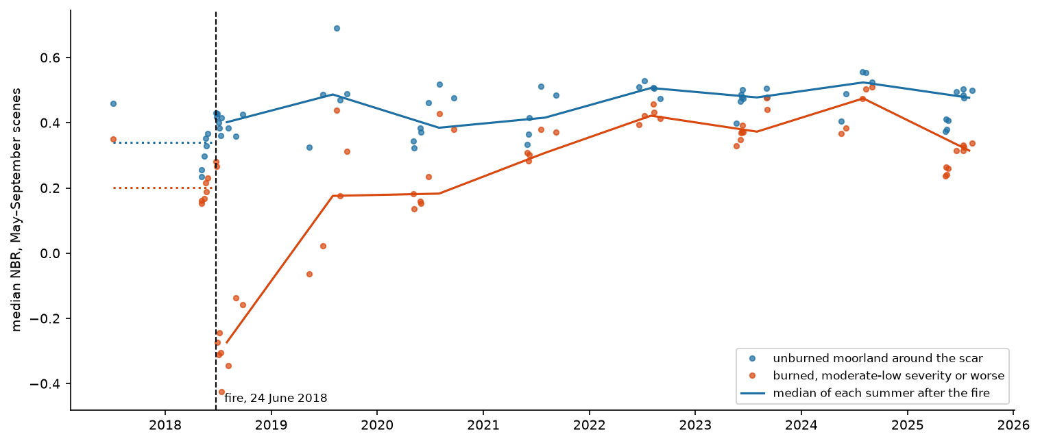

Notice that the area that burned had a lower NBR than its surroundings before the fire (0.202 against 0.341). It was drier, with more bare peat and older heather, which may be part of the reason it burned. So “recovered” here means the gap returned to 0.133, not that the two lines met. That happened in 2021, three summers after the fire. In 2022 and 2024 the gap was smaller than before the fire, which is typical of grasses and young vegetation that green up more strongly than old heather. The wider gap in 2025, a dry year, shows that single summers should not be over-interpreted. NBR measures the canopy only; peat and moss recovery take far longer and need field surveys.

Limitations and honest caveats

• The thresholds come from forests. Key and Benson calibrated the dNBR classes against the Composite Burn Index in North American conifer forests. On moorland, “high severity” means that the vegetation was removed and the surface blackened. It does not measure how deep the fire burned into the peat, which is what matters most for carbon loss and recovery. Treat the classes as relative and calibrate them with field data where you can.
• Drought and land management. The summer of 2018 was exceptionally dry, and grass cutting is common in the valleys. Both create false “low severity” pixels. A short gap between images, an offset from local unburned ground and a connected perimeter keep this under control, but they do not remove it.
• Pixel size. At 20 m, narrow burned strips, firebreaks and small spot fires blur into their surroundings, and the perimeter edges are uncertain by about one pixel. Along 28.9 km of edge, one pixel is about 58 ha.
• Smoke and cloud. Images taken while a fire is still burning can contain smoke, which SCL often misses. Thick smoke is bright in the visible bands but nearly transparent in B12, so it can lower NBR or partly hide the burn. Check your images visually before trusting them.
• Reflectance consistency. Mixing processing baselines needs the offset described in Step 2. Mixing Sentinel-2 with Landsat needs band harmonisation, because the NIR and SWIR bands are slightly different.
• NBR saturates. Once the canopy is gone, there is little left to measure, so dNBR cannot separate a severe surface fire from one that also burned deep into the soil.

Frequently asked questions

How do you calculate dNBR in Python?

Read the NIR and SWIR2 bands for a pre-fire and a post-fire image on the same grid (B8A and B12 for Sentinel-2, bands 5 and 7 for Landsat 8 and 9), convert them to reflectance, and compute NBR = (NIR − SWIR2) / (NIR + SWIR2) for each date with NumPy. dNBR is nbr_pre - nbr_post. Mask cloud, shadow and water first, and subtract the median dNBR of nearby unburned land as an offset.

What are the dNBR burn severity classes?

The USGS classes from Key and Benson (2006) are: enhanced regrowth below −0.101, unburned −0.101 to 0.099, low severity 0.100 to 0.269, moderate-low 0.270 to 0.439, moderate-high 0.440 to 0.659 and high severity 0.660 and above. Many sources quote them multiplied by 1000 (100, 270, 440 and 660). They are a starting point; the best thresholds depend on the vegetation and should be checked against field data.

Which Sentinel-2 bands are used for NBR?

B8A (narrow near-infrared, 865 nm) and B12 (shortwave infrared, 2190 nm), both at 20 m resolution. Some workflows use B8 (broad NIR, 10 m) instead of B8A; the results are very similar but B8 has to be resampled to 20 m to match B12. NBR2, which uses B11 and B12, is sometimes added to detect post-fire changes in soil moisture.

What is the difference between dNBR and RdNBR?

dNBR is the absolute change in NBR. RdNBR divides it by the square root of the pre-fire NBR, so it measures the change relative to how much vegetation there was. RdNBR makes fires in sparse and dense vegetation more comparable, but it becomes unstable where pre-fire NBR is close to zero, and its published thresholds are for forests.

How soon after a fire should the post-fire image be taken?

As soon as the fire is out and a clear image is available, usually within a few weeks, for an initial assessment. Waiting until the next growing season (an extended assessment) shows which vegetation survived, which is useful in forests. In grassland and moorland, regrowth starts within weeks, so a late image will understate severity.

Can I use Landsat instead of Sentinel-2?

Yes. Landsat 8 and 9 Collection 2 Level-2 surface reflectance works in the same way with bands 5 (NIR) and 7 (SWIR2) at 30 m, and the archive goes back to the 1980s with Landsat 5 and 7. Our Landsat land surface temperature tutorial shows how to read Landsat Level-2 data from the Planetary Computer and mask clouds with QA_PIXEL.

Next steps

• Add the terrain: burned slopes erode faster. Derive slope and aspect for the scar with raster terrain analysis in rasterio.
• See how the fire affected water downstream: the reservoirs in monitoring reservoir water quality with Sentinel-2 drain the same kind of peat moorland.
• Repeat the analysis for another fire, such as the 2018 Winter Hill fire in Lancashire or a large forest fire, and compare the dNBR and RdNBR classes.
• Publish the perimeter and severity map on an interactive Folium web map.
• If you are new to STAC and Sentinel-2, start with measuring Lake Mead’s shoreline with Sentinel-2 and STAC. When cloud blocks the optical images, Sentinel-1 SAR can still see the ground.

Data and licences

• Sentinel-2 L2A: contains modified Copernicus Sentinel data 2017–2025, processed by ESA. Accessed as Cloud Optimised GeoTIFFs from the Microsoft Planetary Computer on 17 October 2026.
• References: Key, C. H. and Benson, N. C. (2006), “Landscape Assessment: Ground measure of severity, the Composite Burn Index; and Remote sensing of severity, the Normalized Burn Ratio”, in FIREMON: Fire Effects Monitoring and Inventory System, USDA Forest Service RMRS-GTR-164-CD; Miller, J. D. and Thode, A. E. (2007), “Quantifying burn severity in a heterogeneous landscape with a relative version of the delta Normalized Burn Ratio (dNBR)”, Remote Sensing of Environment 109(1); Parks, S. A. et al. (2014), “A new metric for quantifying burn severity: the relativized burn ratio”, Remote Sensing 6(3); UN-SPIDER Knowledge Portal, “Recommended practice: burn severity mapping”.
• Code: burn_severity_dnbr.py, tested with Python 3.12.0, pystac-client 0.9.0, planetary-computer 1.0.0, rasterio 1.5.2, numpy 2.5.4, scipy 1.18.1 and pandas 3.0.6.