Land surface temperature from Landsat in Python: mapping London's urban heat island
Calculate land surface temperature from Landsat 8 and 9 Collection 2 Level-2 data in Python: ST_B10 scale and offset, QA_PIXEL cloud masking, LST by land cover and NDVI, an urban-rural transect, hotspots with OpenStreetMap and an honest comparison with air temperature, for London in the July 2022 heatwave.
- Level
- Intermediate
- Tested with
- Python 3.12
- Source code
- Download scripts
Key takeaways
- Landsat Collection 2 Level-2 already contains land surface temperature in band ST_B10. Kelvin = DN × 0.00341802 + 149.0; subtract 273.15 for degrees Celsius.
- Mask fill, cloud, dilated cloud, cirrus, shadow and snow with the QA_PIXEL bits, buffer the mask, and drop water (bit 7) before computing statistics.
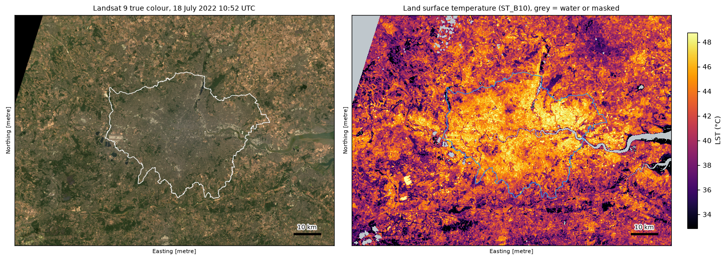
- On 18 July 2022 at 10:52 UTC, built-up land in Greater London had a median surface temperature of 45.8 °C, 5.1 °C warmer than rural grass and cropland around the city. Each 0.1 increase in NDVI was linked to 0.9 °C cooler surfaces.
- Dry grass was nearly as hot as roofs and roads in the drought: two of London's ten largest hotspots were open grassland.
- Land surface temperature is not air temperature. Near four weather stations, the surface was 7–13 °C hotter than the air at the same moment.
Before you start
- Comfortable with NumPy, pandas and rasterio (the Sentinel-2 Lake Mead tutorial introduces STAC searches and Cloud Optimised GeoTIFFs)
- Python 3.10+ with pystac-client, planetary-computer, rasterio, numpy, scipy, pandas, geopandas, osmnx, requests and matplotlib
- An internet connection: Landsat and WorldCover are streamed from the Microsoft Planetary Computer and need no account or API key
Short answer: to calculate land surface temperature from Landsat in Python, find a clear Landsat 8 or 9 Collection 2 Level-2 scene with a STAC search and read its surface temperature band ST_B10. Apply the scale factor and offset (kelvin = DN × 0.00341802 + 149.0) and subtract 273.15 to get °C. Mask fill, cloud, cloud shadow and snow with the QA_PIXEL bits, and drop water. The atmospheric and emissivity corrections are already done by the USGS, so there is no need to compute brightness temperature or emissivity yourself. To measure the urban heat island, compare the median LST of built-up land with that of rural land nearby. For London on 18 July 2022 the difference was 5.1 °C.
On 18 and 19 July 2022, the Met Office issued its first ever red warning for extreme heat, and on 19 July the UK passed 40 °C for the first time; Heathrow reached 40.2 °C. Neither Landsat 8 nor Landsat 9 passed over London on a clear 19 July, but Landsat 9 did on the morning of 18 July, with only 0.72% cloud in the scene. That image is our case study: how hot London’s surfaces became, which places were hottest and why, and what a satellite thermal image can and cannot tell you about the heat people feel.
You will learn how to:
- search the Landsat Collection 2 Level-2 archive on the Microsoft Planetary Computer and choose a clear scene;
- turn ST_B10 digital numbers into kelvin and °C with the scale factor and offset (the LST calculation);
- mask cloud, shadow and water with QA_PIXEL bits, and read the per-pixel uncertainty from ST_QA;
- summarise LST by ESA WorldCover land cover and by NDVI;
- measure the surface urban heat island intensity and draw an urban–rural transect;
- find hotspots and put them in context with OpenStreetMap land use and Nominatim place names;
- compare LST with air temperature from weather stations, honestly.
All outputs below are real results from lst_urban_heat_island.py, run on 17 October 2026 with Python 3.12, pystac-client 0.9.0, planetary-computer 1.0.0, rasterio 1.5.2 and osmnx 2.1.1.
What Landsat measures, and what it does not
Everything warmer than absolute zero emits thermal infrared radiation, and hotter surfaces emit more. The Thermal Infrared Sensor (TIRS) on Landsat 8 and 9 measures this radiation at around 10.9 µm (band 10) from 705 km up. The USGS then turns it into a surface temperature product. The algorithm corrects for the atmosphere between the ground and the satellite, using reanalysis data on water vapour and temperature, and for emissivity, using the ASTER Global Emissivity Database adjusted with NDVI. The result, in Level-2 band ST_B10, is the radiative skin temperature of whatever the sensor sees from above: roofs, roads, grass, bare soil or the top of tree canopies.
That is not the same as the air temperature measured by a thermometer in a shaded screen 1.25–2 m above grass. On a sunny summer day, a dark roof or a dry field can be 20 °C hotter than the air above it. We return to this in Step 8.
Two more things to keep in mind:
- Resolution. TIRS pixels are 100 m across. The USGS resamples ST_B10 to the 30 m grid of the other bands, but the detail is still roughly 100 m.
- Timing. Landsat 8 and 9 cross the equator at about 10:00 local solar time, which over London means around 10:50 UTC (11:50 British Summer Time). This is one morning snapshot, not the afternoon peak and not the night, when the urban heat island in air temperature is strongest.
Step 1: find a clear Landsat 8/9 scene on a hot day
The Microsoft Planetary Computer hosts Landsat Collection 2 Level-2 as Cloud Optimised GeoTIFFs. We search the summer of 2022 for scenes over London with less than 10% cloud:
STAC_URL = "https://planetarycomputer.microsoft.com/api/stac/v1"AOI = (-0.95, 51.15, 0.65, 51.85)    # lon/lat: Greater London plus a rural margin on every sideCENTRE = (-0.1276, 51.5072)           # Trafalgar Square / Charing Cross, the traditional centre of London
catalog = pystac_client.Client.open(STAC_URL, modifier=planetary_computer.sign_inplace)search = catalog.search(collections=["landsat-c2-l2"], bbox=AOI, datetime="2022-06-01/2022-08-31", query={"platform": {"in": ["landsat-8", "landsat-9"]}, "eo:cloud_cover": {"lt": 10}})summer = sorted(search.items(), key=lambda i: i.datetime)item = next(it for it in summer if it.id == "LC09_L2SP_201024_20220718_02_T1")st = item.assets["lwir11"].extra_fields["raster:bands"][0]2022-07-10 10:52 UTC landsat-8 path/row 201/024 cloud 1.47%2022-07-10 10:53 UTC landsat-8 path/row 201/025 cloud 0.52%2022-07-11 10:46 UTC landsat-9 path/row 200/024 cloud 0.93%2022-07-11 10:46 UTC landsat-9 path/row 200/025 cloud 0.02%2022-07-18 10:52 UTC landsat-9 path/row 201/024 cloud 0.72%2022-07-18 10:52 UTC landsat-9 path/row 201/025 cloud 5.60%2022-08-10 10:58 UTC landsat-9 path/row 202/024 cloud 0.03%2022-08-11 10:52 UTC landsat-8 path/row 201/024 cloud 0.01%2022-08-12 10:46 UTC landsat-9 path/row 200/024 cloud 0.02%2022-08-12 10:46 UTC landsat-9 path/row 200/025 cloud 0.01%
using LC09_L2SP_201024_20220718_02_T1: 18 July 2022 10:52 UTC, sun elevation 56.2 deg, EPSG:32631ST_B10 (asset 'lwir11'): scale 0.00341802, offset 149, unit kelvin, nodata 0The summer of 2022 was unusually clear, with ten scenes under 10% cloud. Path/row 201/024 covers all of Greater London in one scene. On the Planetary Computer the surface temperature band is the asset lwir11, and the STAC metadata gives its scale and offset, so you can check them rather than copying them from a web page.
Step 2: the LST calculation, from digital numbers to °C
We read a 114 × 83 km window of the scene in its own projection (UTM zone 31N), so nothing is resampled. Collection 2 Level-2 stores both temperature and reflectance as integers that need a scale factor and an offset:
dn = raw["lwir11"]lst_k = np.where(dn > 0, dn * 0.00341802 + 149.0, np.nan)       # Collection 2 Level-2 ST scale and offsetlst = lst_k - 273.15                                             # kelvin to degrees Celsiusst_unc = np.where(raw["qa"] >= 0, raw["qa"] * 0.01, np.nan)     # ST_QA: uncertainty in kelvin

def sr(band: str) -> np.ndarray:    """Collection 2 surface reflectance: DN * 0.0000275 - 0.2."""    v = raw[band]    return np.where(v > 0, v * 2.75e-5 - 0.2, np.nan)

red, nir = sr("red"), sr("nir08")with np.errstate(divide="ignore", invalid="ignore"): ndvi = (nir - red) / (nir + red)grid 3812 x 2753 pixels of 30 m (114 x 83 km)DN 39298..54444 -> 283.3..335.1 K -> 10.2..61.9 degCThe coldest pixels, at 10 °C, are water and small cloud tops that the mask in Step 3 removes; the hottest, at 62 °C, are a handful of individual pixels, most likely over industrial roofs or yards. A digital number of 0 is fill and must become NaN before scaling; otherwise it turns into 149 K (−124 °C).
Step 3: mask cloud, shadow and water with QA_PIXEL
The QA_PIXEL band packs several flags into the bits of one 16-bit integer. We test each bit with a shift and a bitwise AND:
qa = raw["qa_pixel"]bit = lambda b: (qa >> b) & 1 == 1 # noqa: E731QA_BITS = {"fill": 0, "dilated cloud": 1, "cirrus": 2, "cloud": 3, "cloud shadow": 4, "snow": 5, "clear": 6, "water": 7}for name, b in QA_BITS.items(): print(f"QA_PIXEL bit {b} ({name}): {bit(b).mean():.2%}")bad = bit(0) | bit(1) | bit(2) | bit(3) | bit(4) | bit(5)bad = ndimage.binary_dilation(bad, iterations=3) # 90 m buffer: thermal pixels are really 100 mwater = bit(7)ok = ~bad & ~water & np.isfinite(lst)QA_PIXEL bit 0 (fill): 1.73%QA_PIXEL bit 1 (dilated cloud): 0.05%QA_PIXEL bit 2 (cirrus): 0.00%QA_PIXEL bit 3 (cloud): 0.04%QA_PIXEL bit 4 (cloud shadow): 0.10%QA_PIXEL bit 5 (snow): 0.00%QA_PIXEL bit 6 (clear): 98.19%QA_PIXEL bit 7 (water): 1.08%usable land pixels: 96.6% | ST_QA uncertainty over land: median 2.06 K, 95th pct 2.94 KTwo details matter for thermal data in particular:
- Buffer the mask. A cloud cools the thermal pixels around it, because each 30 m pixel is resampled from a 100 m measurement. We grow the mask by three pixels (90 m).
- Water. Water is much cooler than land in the day and has a different emissivity, so leaving it in drags down every average. Bit 7 removes the Thames, reservoirs and lakes.
The ST_QA band (asset qa) gives an uncertainty for every pixel, in hundredths of a kelvin. Here the median is 2.06 K: any single pixel’s temperature is only known to within about ±2 °C. Differences between large areas are much more reliable than individual pixel values.
Step 4: LST by land cover and NDVI
To see what is hot, we combine LST with the ESA WorldCover 2021 10 m land-cover map, also on the Planetary Computer. We warp it to the 30 m Landsat grid with mode resampling, which keeps the most common class in each pixel. The Greater London boundary comes from OpenStreetMap through osmnx:
ox.geocode_to_gdf("Greater London, England")[["geometry"]].to_file(gl_file, driver="GPKG")gl = gpd.read_file(gl_file).to_crs(CRS)in_gl = rasterio.features.geometry_mask(gl.geometry, (HEIGHT, WIDTH), TRANSFORM, invert=True)
wc = np.zeros((HEIGHT, WIDTH), dtype="uint8")for wi in catalog.search(collections=["esa-worldcover"], bbox=AOI,                         query={"esa_worldcover:product_version": {"eq": "2.0.0"}}).items():    with rasterio.open(wi.assets["map"].href) as src, WarpedVRT(src, crs=CRS, transform=TRANSFORM, width=WIDTH,                                                               height=HEIGHT, resampling=Resampling.mode) as vrt:        tile = vrt.read(1)    wc = np.where(tile > 0, tile, wc)
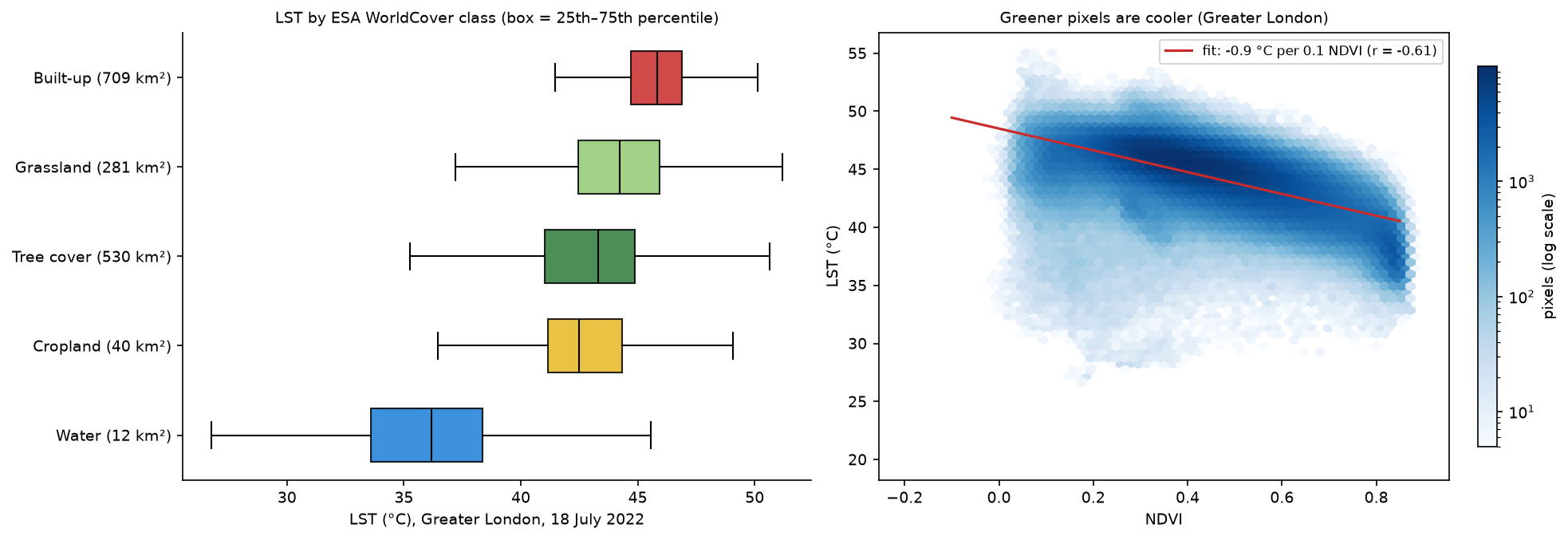
for code, name in WC.items(): m = ok & in_gl & (wc == code) if m.sum() * PX_KM2 < 5: # skip classes covering less than 5 km2 of London continue v = lst[m] rows.append({"land cover": name, "km2": round(m.sum() * PX_KM2, 1), "median_C": np.median(v), "p10_C": np.percentile(v, 10), "p90_C": np.percentile(v, 90), "median_NDVI": np.median(ndvi[m])})land cover km2 median_C p10_C p90_C median_NDVI Built-up 709.2 45.84 43.53 47.73 0.33 Grassland 280.6 44.24 40.84 47.38 0.48Tree cover 529.5 43.31 38.71 46.00 0.60 Cropland 39.5 42.49 39.98 45.99 0.33 Water 12.2 36.17 30.93 40.32 0.29Built-up land is the hottest class, as expected, but by less than you might think: grassland is only 1.6 °C cooler. After a dry spring and early summer, London’s parks and verges were brown, and dry grass heats up almost as much as tarmac because it has no water left to evaporate. Tree cover is cooler again, and its 10th percentile, 38.7 °C, is 4.8 °C below that of built-up land: shade and transpiration both work. (The “water” here is the 12 km² that WorldCover maps as water but QA_PIXEL did not flag, mostly river edges and small ponds.)
The relationship with NDVI is clearer still:
slope, intercept = np.polyfit(ndvi[gl_ok], lst[gl_ok], 1)r = np.corrcoef(ndvi[gl_ok], lst[gl_ok])[0, 1] ndvi_from n median_Cbin1 -0.1 235 39.092 0.0 29871 45.713 0.1 106285 46.284 0.2 220600 46.385 0.3 381107 45.816 0.4 369689 45.007 0.5 279661 43.988 0.6 175329 42.719 0.7 109904 41.0010 0.8 74389 38.45linear fit: LST = 48.5 -9.4 x NDVI (r = -0.61, -0.9 C per 0.1 NDVI)Every 0.1 increase in NDVI goes with surfaces about 0.9 °C cooler, and the greenest pixels (NDVI above 0.8, mostly woodland) are about 8 °C cooler than the least green. The relationship is not linear: below an NDVI of about 0.3, LST hardly changes, and above 0.6 it drops steeply. The few pixels below NDVI 0 are cooler because many are wet: the edges of water bodies.
Step 5: measure the surface urban heat island
The surface urban heat island (SUHI) intensity is usually defined as the difference between the LST of urban and rural land. The answer depends heavily on what you call “rural”, so we make the choice explicit: grass and cropland more than 5 km outside Greater London, with less than 5% built-up land within about 1 km:
built_1km = ndimage.uniform_filter((wc == 50).astype("float32"), size=33) # built-up share within ~1 kmdist_gl_km = ndimage.distance_transform_edt(~in_gl) * 0.03rural = ok & ~in_gl & (dist_gl_km > 5) & np.isin(wc, [30, 40]) & (built_1km < 0.05)urban = ok & in_gl & (wc == 50)suhi = np.median(lst[urban]) - np.median(lst[rural])urban: built-up pixels in Greater London, 709 km2, median LST 45.8 Crural: grass/cropland > 5 km outside London with < 5% built-up within 1 km, 2,702 km2, median LST 40.8 Csurface urban heat island intensity (median urban - median rural): 5.1 Call land within 5 km of Charing Cross: median LST 45.0 CLondon’s built-up surfaces were 5.1 °C hotter than the rural land around the city at 10:52 UTC. Interestingly, the land within 5 km of Charing Cross, at 45.0 °C, was slightly cooler than built-up land across Greater London as a whole. Central London has large parks, the river, tall buildings that shade the streets, and many light-coloured roofs, while some of the hottest surfaces are in the outer boroughs, as Step 7 shows.
If you compare with forest instead of grass and cropland, the intensity rises; if you compare with dry arable land, it falls. Published SUHI values for the same city on the same day can differ by several degrees for this reason alone, so always state your rural reference.
Step 6: draw an urban–rural transect
A transect shows how temperature changes across the city. We take the row of pixels through Charing Cross, from Berkshire in the west to Essex in the east, and smooth it with a 1 km running median:
cx, cy = to_utm.transform(*CENTRE)row = int((y1 - cy) // 30)tx = x0 + 15 + np.arange(WIDTH) * 30t_lst = pd.Series(np.where(ok[row], lst[row], np.nan))t_ndvi = pd.Series(np.where(ok[row], ndvi[row], np.nan))t_lst_s = t_lst.rolling(31, center=True, min_periods=10).median() # ~1 km running mediant_ndvi_s = t_ndvi.rolling(31, center=True, min_periods=10).median()km = (tx - cx) / 1000transect length 114 km; Greater London boundary crossed at -25.1, +25.5 kmrural west (Berkshire) -60 to -40 km: median LST 42.1 C, NDVI 0.50central London -5 to +5 km: median LST 43.0 C, NDVI 0.24rural east (Essex) +40 to +60 km: median LST 43.2 C, NDVI 0.35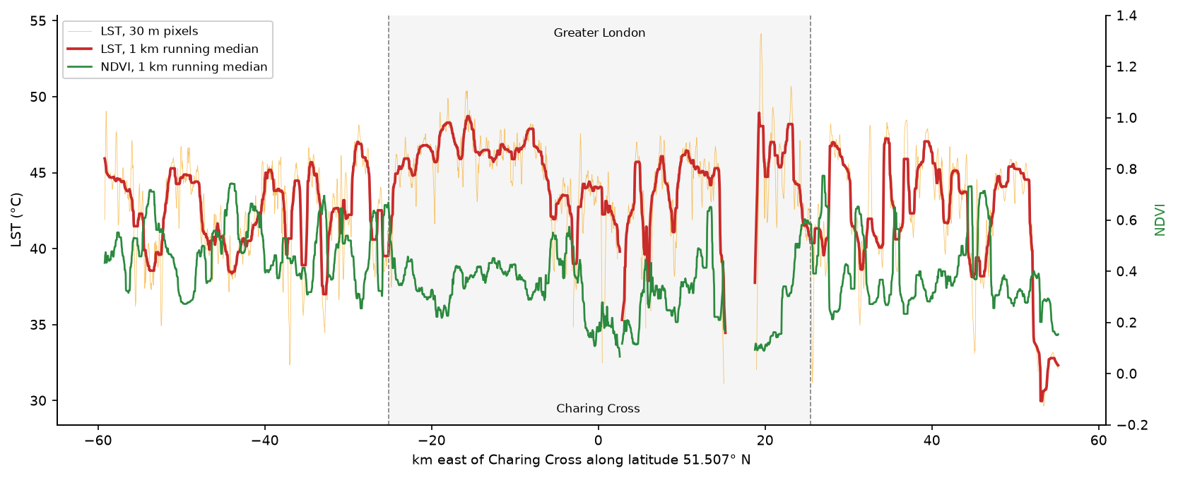
The transect is a useful reality check. Inside Greater London, NDVI stays low for 50 km and LST is high for most of that distance, dipping at parks and the river. Outside, LST swings by 10 °C between woods and fields. The rural west, with more woodland (NDVI 0.50), is cooler than central London, but the rural east, with dry arable fields and an NDVI of only 0.35, is slightly hotter. A single transect can tell any story you want, so use it to illustrate, and base numbers on area statistics such as the SUHI in Step 5. The sharp drop at the far eastern end is where the line reaches the wet margins of the Thames estuary.
Step 7: find hotspots and name them with OpenStreetMap
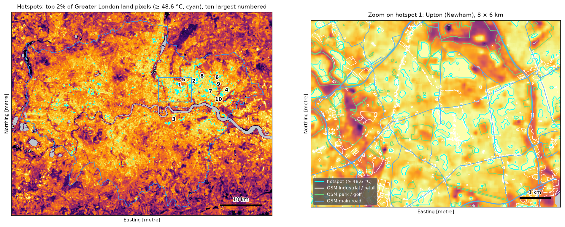
We define hotspots as the hottest 2% of land pixels in Greater London, clean them with a morphological closing, label connected patches with scipy.ndimage, and keep the ten largest. Nominatim, the OpenStreetMap geocoder, then gives each one a place name. We send at most one request per second with a descriptive User-Agent, as the Nominatim usage policy requires, and cache the answers:
thr = np.percentile(lst[gl_ok], 98)hot = gl_ok & (lst >= thr)hot = ndimage.binary_closing(hot, iterations=1) & gl_oklab, n = ndimage.label(hot)sizes = ndimage.sum(hot, lab, index=np.arange(1, n + 1))order = np.argsort(sizes)[::-1][:10] + 1for k, lid in enumerate(order, 1): m = lab == lid rr, cc = np.nonzero(m) j = np.argmax(lst[rr, cc]) hx, hy = x0 + (cc[j] + 0.5) * 30, y1 - (rr[j] + 0.5) * 30 lon, lat = to_ll.transform(hx, hy) key = f"{lat:.5f},{lon:.5f}" if key not in names: resp = requests.get("https://nominatim.openstreetmap.org/reverse", headers=HEADERS, timeout=30, params={"lat": lat, "lon": lon, "format": "jsonv2", "zoom": 17}) names[key] = resp.json() time.sleep(1.1) # Nominatim usage policy: at most one request a secondFor each hotspot we also record the share of built-up, grass and tree pixels from WorldCover, and the median NDVI.
threshold 48.6 C; 1,138 patches, 160 of at least 5 ha rank area_ha max_C mean_C place borough near built_% grass_% tree_% NDVI 1 88.1 51.6 49.1 Upton Newham Chaucer Road 99 0 1 0.23 2 85.7 50.1 49.0 Seven Kings Redbridge Ilford Lane 96 1 2 0.24 3 54.0 51.7 49.8 Blackheath Lewisham Prince Charles Road 1 98 0 0.31 4 54.0 54.0 50.1 South Hornchurch Havering Ford Lane 21 74 4 0.33 5 44.6 52.2 49.6 Manor Park Newham Capel Road 0 97 3 0.36 6 44.6 55.7 49.8 Becontree Heath Barking and Dagenham 39 61 0 0.29 7 42.9 54.9 49.8 Scrattons Farm Barking and Dagenham Goresbrook Road 56 38 6 0.26 8 34.7 49.8 49.1 Seven Kings Redbridge Pembroke Road 96 2 2 0.27 9 34.1 51.2 49.5 Dagenham Barking and Dagenham Manchester Way 56 44 1 0.24 10 33.8 57.8 51.5 Scrattons Farm Barking and Dagenham Ford Dagenham 99 0 1 0.11ten largest hotspots together: 517 ha, 60% built-up, 38% grass or crops, 2% trees (WorldCover)All ten are in east and south-east London, and they fall into three groups:
- Dense terraced housing with few trees (1, 2 and 8): Upton and Manor Park in Newham, and Seven Kings in Ilford. These are almost entirely built-up, with a median NDVI below 0.3.
- Industry: hotspot 10 is the Ford Dagenham plant, with the highest temperature in London’s top ten, 57.8 °C, and the lowest NDVI, 0.11. Large, flat, dark roofs and yards are the classic urban hotspot.
- Dry open grassland (3, 4, 5 and 6): Blackheath, the grassland of Wanstead Flats next to Capel Road in Manor Park, and open land in Havering and Barking and Dagenham are 61–98% grass. Parched grass in full sun was as hot as any roof.
Together, the ten largest hotspots are 60% built-up and 38% grass or crops. Only 2% is tree cover. Reverse geocoding returns the nearest named road or feature, so treat the “near” column as an address for finding the place, not a description of it.
To see the fine detail, we download OpenStreetMap land use, parks and main roads for an 8 × 6 km box around hotspot 1 with osmnx, rasterise each tag, and compare temperatures:
tags = {"landuse": ["residential", "industrial", "commercial", "retail", "railway"], "leisure": ["park", "golf_course"], "highway": ["motorway", "trunk", "primary"]}osm = ox.features_from_bbox((zoom_ll[0][0], zoom_ll[1][0], zoom_ll[0][1], zoom_ll[1][1]), tags)for col, vals in (("landuse", ["residential", "industrial", "commercial", "retail"]), ("leisure", ["park", "golf_course"])): for v in vals: polys = osm[(osm[col] == v) & osm.geom_type.isin(["Polygon", "MultiPolygon"])] mm = rasterio.features.geometry_mask(polys.geometry, (HEIGHT, WIDTH), TRANSFORM, invert=True)[zr] & zone_okOpenStreetMap features in the 8 x 6 km box around hotspot 1: 4,137OSM tag km2 median LST share of hotspot pixelslanduse=residential 21.10 47.4 C 38%landuse=industrial 1.71 45.8 C 2%landuse=commercial 1.00 46.8 C 2%landuse=retail 1.71 47.8 C 8%leisure=park 6.28 45.5 C 13%leisure=golf_course 0.61 43.3 C 0%In this part of Newham and Redbridge, residential land (47.4 °C) and retail parks (47.8 °C) were the hottest uses, and residential areas held 38% of the hotspot pixels. Parks were cooler on average, at 45.5 °C, but still contained 13% of the hotspot pixels: their open, sun-baked grass. The golf course, with watered greens and more trees, was the coolest at 43.3 °C.
Step 8: land surface temperature is not air temperature
Finally, we compare LST with the air temperature measured at four weather stations at the time of the overpass. We use the free hourly data from Meteostat, which redistributes observations from national weather services, and take the median LST within about 1 km of each station:
STATIONS = {"03772": ("Heathrow", 51.4833, -0.45), "03672": ("Northolt", 51.55, -0.4167), "03781": ("Kenley", 51.30, -0.0833), "EGKB0": ("Biggin Hill", 51.3167, 0.0333)}for sid, (name, lat, lon) in STATIONS.items(): f = CACHE / f"meteostat_{sid}_2022.csv.gz" if not f.exists(): f.write_bytes(requests.get(f"https://bulk.meteostat.net/v2/hourly/2022/{sid}.csv.gz", headers=HEADERS, timeout=60).content) obs = pd.read_csv(f, header=None, usecols=[0, 1, 2], names=["date", "hour", "temp"]) t = obs[(obs["date"] == "2022-07-18") & (obs["hour"].isin([10, 11]))]["temp"] sx, sy = to_utm.transform(lon, lat) rr, cc = int((y1 - sy) // 30), int((sx - x0) // 30) win = (slice(rr - 16, rr + 17), slice(cc - 16, cc + 17)) # ~1 km box: station coordinates are rounded station air_10UTC_C air_11UTC_C LST_median_1km_C LST_grass_median_C LST_minus_air Heathrow 31.3 33.7 46.5 46.2 12.8 Northolt 31.8 33.3 46.2 45.9 12.9 Kenley 29.4 31.2 38.5 40.4 7.3Biggin Hill 30.0 32.0 42.6 43.2 10.6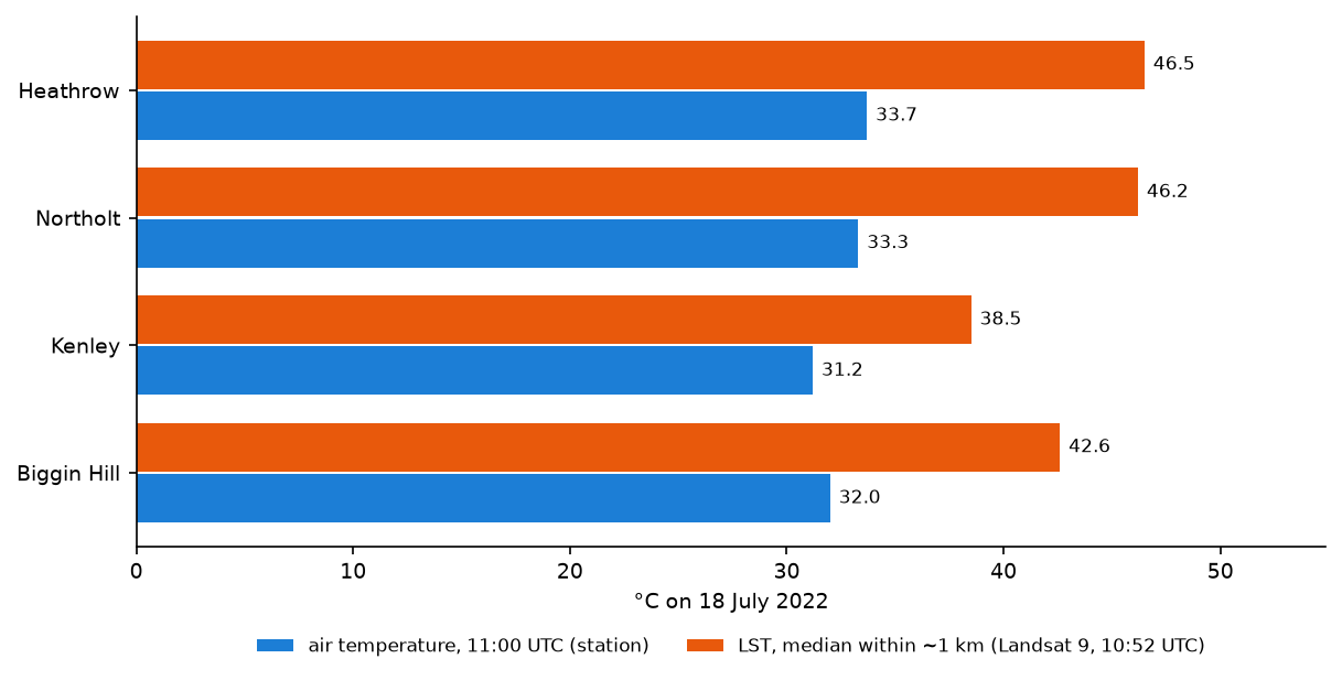
The air was 31–34 °C at 11:00 UTC; the surfaces around the stations were 38.5–46.5 °C. The difference is largest at Heathrow and Northolt, two airfields with large areas of tarmac and dry grass, and smallest at Kenley, an airfield on the wooded North Downs. The air temperatures at the four stations differed by only 2.5 °C, but the LST differed by 8 °C. Wind mixes the air near the ground, while each surface heats up according to its own colour, moisture and exposure to the sun.
Limitations and honest caveats
- One snapshot. Everything here describes 10:52 UTC on 18 July 2022. Afternoon surface temperatures were higher, night-time patterns are very different, and the next clear Landsat image did not come until 10 August.
- Resolution. ST_B10 is a 100 m measurement resampled to 30 m. Small features such as a single roof, a narrow street or a small park are blurred with their surroundings, so pixel-level hotspots are approximate.
- Emissivity and uncertainty. The Collection 2 algorithm estimates emissivity from ASTER data collected around 2000–2008, adjusted with NDVI. Where land use has changed since, or for unusual materials such as metal roofs, the error can exceed the typical 2 K given by ST_QA.
- Viewing geometry. A satellite looking straight down sees roofs and tree tops, not walls and shaded streets. The temperature that people experience in a street canyon is different.
- Rural reference. The SUHI intensity depends on the reference land you choose. Our 5.1 °C is for dry grass and cropland; with woodland as the reference, it would be larger.
- Drought. In 2022 the grass was exceptionally dry. In a wetter summer, parks would be much cooler relative to buildings, and the hotspot ranking would change.
Frequently asked questions
How do you calculate land surface temperature from Landsat in Python?
With Collection 2 Level-2 data, read band ST_B10 (asset lwir11 on the Planetary Computer) with rasterio, set DN 0 to NaN, and apply kelvin = dn * 0.00341802 + 149.0, then celsius = kelvin - 273.15. Mask cloud, shadow, snow and water with QA_PIXEL bits 0–5 and 7. With Level-1 data you would need to convert band 10 to radiance and brightness temperature and correct for emissivity yourself, which is why Level-2 is the easier and better choice.
What is the scale factor for Landsat ST_B10?
For Landsat Collection 2 Level-2, the surface temperature scale factor is 0.00341802 and the offset is 149.0, giving kelvin. Surface reflectance bands use a scale of 0.0000275 and an offset of −0.2. Both values are in the STAC metadata (raster:bands) and in the USGS product guide. Collection 1 used a scale of 0.1 without an offset, so older recipes give wrong results on Collection 2.
What is the difference between land surface temperature and air temperature?
LST is the temperature of the surface itself as seen by a satellite’s thermal sensor, while air temperature is measured in the shade about 1.5 m above the ground. On a sunny day, dry and dark surfaces can be 10–20 °C hotter than the air; at night, surfaces can be cooler than the air. In this tutorial, LST near four London weather stations was 7–13 °C higher than the air temperature at the same time.
How do you measure the urban heat island with satellite data?
Calculate LST, mask cloud and water, classify pixels as urban or rural with a land-cover map such as ESA WorldCover, and subtract the median rural LST from the median urban LST. That gives the surface urban heat island intensity. State how you defined “rural”, because the result depends on it, and remember that it describes surfaces at the time of the overpass, not air temperature.
Why is Landsat LST only available around 11 am?
Landsat 8 and 9 are in sun-synchronous orbits that cross the equator at about 10:00 local solar time, so they always image a given place in the late morning. For other times of day, use ECOSTRESS on the International Space Station, which passes at varying times, or MODIS and Sentinel-3 SLSTR, which observe several times a day between them but with 1 km pixels.
Can I use this method for another city?
Yes. Change the bounding box, the city boundary and the scene ID, and choose a rural reference that suits the region. Look for a clear scene during a heatwave, ideally with low wind. In arid cities, the surroundings may be bare, hot desert, so the surface heat island can be negative in the daytime: the irrigated city is cooler than the desert around it.
Next steps
- Repeat the analysis for the 10 August 2022 scene, or for several summers, and see which hotspots persist.
- Add the terrain and building heights: raster terrain analysis with rasterio shows how to work with elevation grids, and LiDAR point clouds with laspy can give building and tree heights.
- Publish the LST map and hotspots on an interactive Folium web map.
- Combine LST with street networks from OSMnx to find the hottest walking routes, or with census data in GeoPandas to see who lives in the hottest areas.
- Use the same Landsat Level-2 data for wildfires: our burn severity tutorial with dNBR explains NBR, which works with Landsat bands 5 and 7.
- New to STAC? Start with measuring Lake Mead’s shoreline with Sentinel-2 and STAC.
Data and licences
- Landsat 9 Collection 2 Level-2: Landsat data courtesy of the U.S. Geological Survey, public domain. Accessed as Cloud Optimised GeoTIFFs from the Microsoft Planetary Computer on 17 October 2026.
- ESA WorldCover 2021 v200: © ESA WorldCover project 2021 / contains modified Copernicus Sentinel data (2021) processed by the ESA WorldCover consortium, licensed under CC BY 4.0. Accessed from the Microsoft Planetary Computer.
- Greater London boundary, land use and roads, and Nominatim place names: © OpenStreetMap contributors, available under the Open Database Licence (ODbL).
- Hourly weather observations: Meteostat, licensed under CC BY-NC 4.0, from national weather service data. The non-commercial licence applies to the station data only.
- References: USGS (2022), Landsat 8–9 Collection 2 Level 2 Science Product Guide, LSDS-1619; Cook, M. et al. (2014), “Development of an operational calibration methodology for the Landsat thermal data archive and initial testing of the atmospheric compensation component of a land surface temperature (LST) product from the archive”, Remote Sensing 6(11); Zanaga, D. et al. (2022), ESA WorldCover 10 m 2021 v200.
- Code:
lst_urban_heat_island.py, tested with Python 3.12.0, pystac-client 0.9.0, planetary-computer 1.0.0, rasterio 1.5.2, osmnx 2.1.1, numpy 2.5.4 and pandas 3.0.6.
Key terms
- LST
- Land surface temperature: the radiative skin temperature of whatever the satellite sees from above (roofs, roads, grass, tree crowns), estimated from thermal infrared radiation.
- SUHI
- Surface urban heat island: how much warmer the urban surface is than its rural surroundings, measured from satellite LST. It is different from the canopy-layer (air temperature) urban heat island.
- ST_B10
- The Landsat 8/9 Collection 2 Level-2 surface temperature band, derived from the TIRS band 10 at 10.9 µm and stored as scaled integers.
- QA_PIXEL
- The Landsat Collection 2 pixel quality band. Each bit flags a condition such as fill, cloud, cloud shadow, snow or water.
- Emissivity
- How efficiently a surface emits thermal radiation compared with a perfect black body. It is needed to turn brightness temperature into surface temperature; Collection 2 uses ASTER GED and NDVI to estimate it.
- NDVI
- Normalised Difference Vegetation Index, (NIR − red) / (NIR + red). Higher values mean denser, greener vegetation.
Data for this tutorial
- Microsoft Planetary Computer · Landsat Collection 2 Level-2 and ESA WorldCover via STAC
- OpenStreetMap · Greater London boundary, land use and roads; Nominatim place names
Licences and formats for each source are listed in the GIS data sources catalogue.