InSAR time series in Python: Svartsengi inflation cycles validated with GNSS

Short answer: to build an InSAR time series in Python, download a network of short-interval unwrapped interferograms (here 364 COMET LiCSAR Sentinel-1 pairs), reference each one to a stable far-field area, and solve, pixel by pixel, the linear system φ_k = x_j − x_i for the phase x at every acquisition date by weighted least squares (the SBAS method). Check unwrapping errors with phase closure. To validate with GNSS, project the station’s east, north and up positions into the line of sight, d_LOS = E·d_e + N·d_n + U·d_u, using the LOS unit vector, and difference it with a GNSS station in the InSAR reference area.

Part 1 of this series mapped 48 days of uplift at Svartsengi, on Iceland’s Reykjanes Peninsula, and Part 2 modelled the magma reservoir beneath it at about 4–5 km depth. But Svartsengi does not inflate steadily. Since the dyke intrusion of 10 November 2023, magma has accumulated beneath it for weeks or months, then drained into dykes that fed nine eruptions on the Sundhnúkur crater row, and the cycle has started again. One interferogram cannot capture that sawtooth. A time series can.

In this tutorial you will:

1. stream 364 interferograms from the ascending track over 2.5 years and look at the network and its coherence;
2. test the unwrapping with phase closure;
3. write a small-baseline (SBAS) inversion in NumPy that solves 112 dates at 15,577 pixels;
4. map the cumulative uplift between eruptions and the deformation across one eruption;
5. validate the time series against GNSS at SENG, both over the whole period and phase by phase, and test for phase bias;
6. look honestly at what goes wrong: eruptions, atmosphere, the reference, unwrapping and coherence loss over fresh lava and snow.

All results are real outputs of insar_gnss_timeseries.py, run on 21 October 2026 with Python 3.12, NumPy 2.5.4 and pandas 3.0.6.

The data: one track, 364 short pairs

COMET’s LiCSAR system processes every Sentinel-1 acquisition over Reykjanes into interferograms with its nearest few neighbours in time, so the ascending frame 016A_02504_162118 has more than 6,000 of them. We use the ascending track only. The descending frame’s archive stops in February 2026 (Part 1), and a time series must be built from a single geometry: each track measures a different line of sight.

The script lists the frame’s interferogram folders and keeps pairs of up to 24 days between February 2024 and July 2026. For each pair it reads only the window covering the peninsula (HTTP range requests, as in Part 1) and multilooks it: averaging 2 × 4 pixels into one, about 200 m square. Multilooking reduces noise and makes the stack small enough to hold in memory.

LICSAR = "https://gws-access.jasmin.ac.uk/public/nceo_geohazards/LiCSAR_products.public"
FRAME = "016A_02504_162118"                    # Sentinel-1 ascending track 16 over Reykjanes
BASE = f"{LICSAR}/16/{FRAME}"
START, END, MAX_DAYS = "20240201", "20260730", 24   # short-baseline network
BBOX = (-22.80, 63.72, -22.05, 64.05)          # same window as parts 1 and 2
ML = (2, 4)                                    # multilook 2 rows x 4 columns -> about 220 m x 195 m
SENG = (-22.4338, 63.8822)                     # GNSS station at the Svartsengi power station
REF_STATION = "NYLA"                           # GNSS station 18 km NW, inside the InSAR reference area
REF_KM = 15                                    # InSAR reference = land pixels > 15 km from SENG
MIN_COH = 0.25                                 # multilooked coherence needed to use a pixel in a pair
WAVELENGTH = 0.0554658                         # Sentinel-1 C-band wavelength in metres
RAD2MM = -WAVELENGTH / (4 * np.pi) * 1000      # LiCSAR convention: positive = towards the satellite


def read_pair(pair: str):
    """Multilooked unwrapped phase and coherence for one pair, cached in data/pairs/ (None if missing)."""
    f = DATA / "pairs" / f"{pair}.npz"
    if not f.exists():
        url = f"{BASE}/interferograms/{pair}/{pair}.geo"
        try:
            unw, t = read_window(f"{url}.unw.tif")
            coh, _ = read_window(f"{url}.cc.tif")
        except rasterio.errors.RasterioIOError:
            return None                                 # listed, but the files are not (yet) online
        land = unw != 0                                 # 0 = sea or not unwrapped by LiCSAR
        np.savez_compressed(f, unw=multilook(unw, land), coh=multilook(coh / 255, land), t=np.array(t)[:6])
    z = np.load(f)
    return z["unw"], z["coh"], rasterio.Affine(*z["t"])


html = requests.get(f"{BASE}/interferograms/", timeout=60).text
online = sorted(set(re.findall(r'href="(\d{8}_\d{8})/"', html)))
wanted = [p for p in online if p[:8] >= START and p[9:] <= END and days(p) <= MAX_DAYS]
(DATA / "pairs").mkdir(exist_ok=True)
with ThreadPoolExecutor(6) as pool:                    # a few parallel HTTP readers
    res = dict(zip(wanted, pool.map(read_pair, wanted)))
pairs = [p for p in wanted if res[p] is not None]

6,427 interferograms online; 369 of <= 24 days between 20240201 and 20260730; 364 have unwrapped products (30 s to read or load)

Five listed pairs have no unwrapped file and are skipped. We start in February 2024 because, at the time of writing, LiCSAR had no unwrapped products for this frame for the pairs between October 2023 and February 2024, which span the dyke intrusion and the first three eruptions.

Step 1: the network and its design matrix

Let the unknowns be the unwrapped phase x₁, …, x_N−1 at each epoch after the first, relative to the first (x₀ = 0). An interferogram k between epochs i and j measures

φ_k = x_j − x_i + ε_k

where ε_k is noise (atmosphere, decorrelation). Stacking all pairs gives φ = A x, where each row of the design matrix A has +1 in column j and −1 in column i. This is the formulation of Berardino et al. (2002). If the network is connected, A has full column rank and the least-squares solution is unique; if it splits into separate groups of dates, A is rank-deficient and the groups cannot be tied together.

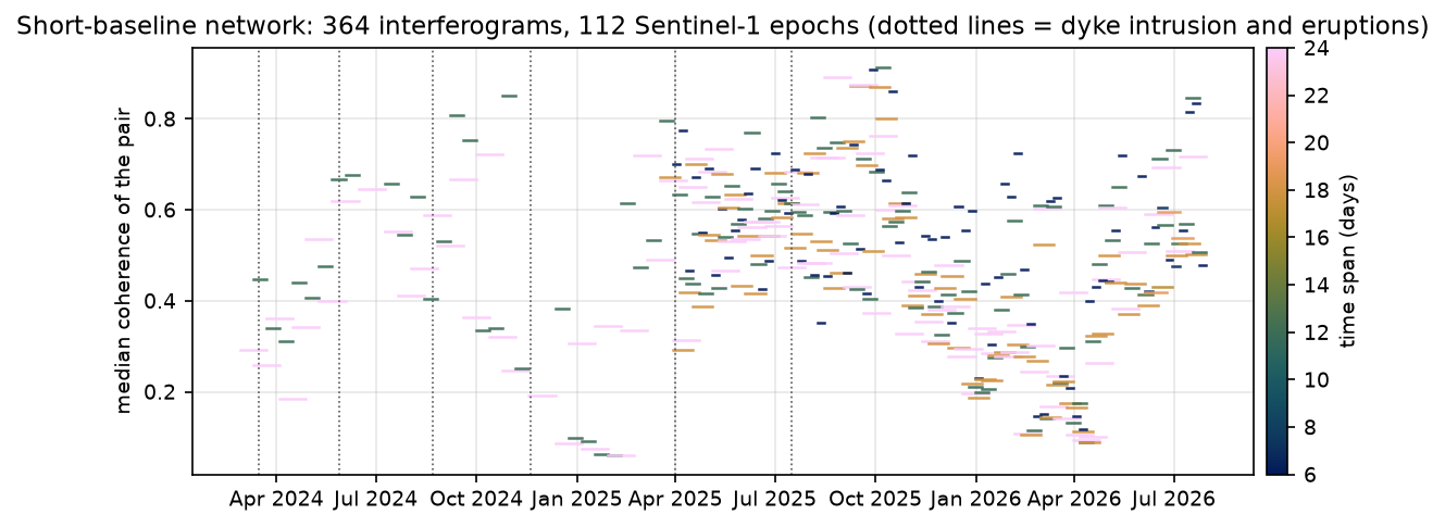
epochs = sorted({p[:8] for p in pairs} | {p[9:] for p in pairs})
idx = {e: i for i, e in enumerate(epochs)}
events = [e for e in EVENTS if epochs[0] < e.replace("-", "") < epochs[-1]]   # eruptions inside the series
A = np.zeros((len(pairs), len(epochs) - 1))         # unknowns: phase at each epoch after the first
for k, p in enumerate(pairs):
    A[k, idx[p[9:]] - 1] = 1
    if idx[p[:8]] > 0:
        A[k, idx[p[:8]] - 1] = -1
spans = pd.Series([days(p) for p in pairs]).value_counts().sort_index()
gaps = np.diff(pd.to_datetime(epochs).values).astype("timedelta64[D]").astype(int)
print(f"{len(pairs)} pairs between {epochs[0]} and {epochs[-1]} -> {len(epochs)} epochs")
print("pairs by time span (days): " + ", ".join(f"{d}: {n}" for d, n in spans.items()))
print(f"design matrix {A.shape}, rank {np.linalg.matrix_rank(A)} (needs {len(epochs) - 1}: one connected network)")

364 pairs between 20240228 and 20260730 -> 112 epochs
pairs by time span (days): 5: 2, 6: 74, 7: 3, 12: 104, 13: 2, 17: 1, 18: 74, 19: 3, 24: 101
design matrix (364, 111), rank 111 (needs 111: one connected network)
epoch spacing: median 6 days, longest 24 days (20240615 to 20240709)

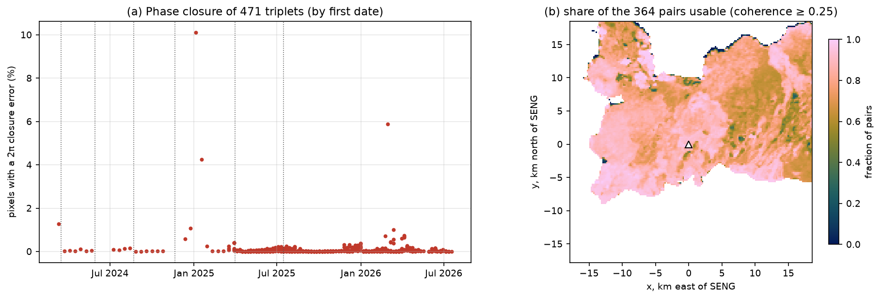
364 interferograms x 165 x 187 pixels (0.004 x 0.002 deg, about 196 m x 221 m)
median coherence per pair: 0.49 (range 0.06-0.91); lowest 20250129_20250222
median coherence in Dec-Mar pairs 0.30 vs Jun-Sep pairs 0.59 (snow)

The network is connected (rank 111 of 111), with 364 equations for 111 unknowns, so it is about three times redundant. Sentinel-1 has acquired every 12 days over Iceland, and every 6 days since Sentinel-1C joined in 2025, which is why the epoch spacing drops in the second half of the series.

Coherence has a clear seasonal cycle: the median coherence of December–March pairs is 0.30, against 0.59 in June–September. Snow cover changes the scattering surface between acquisitions, and is a major limitation for InSAR in Iceland.

Referencing each interferogram

Each interferogram has its own arbitrary phase offset, and long-wavelength errors from orbits, the ionosphere and the troposphere. Before the inversion, the script fits a plane to the land more than 15 km from SENG in each interferogram and subtracts it, then sets the median of that far field to zero. That makes the reference for the whole time series the far field of the peninsula, about where the deformation from a 4–5 km deep source has decayed to a few per cent of its peak (Part 2).

use_obs = np.isfinite(unw) & (coh >= MIN_COH)
for k in range(n_ifg):
    f = far & use_obs[k]
    unw[k] = deramp(unw[k], f, X, Y)
    unw[k] -= np.nanmedian(unw[k][f])

reference: 4,879 land pixels > 15 km from SENG; plane removed from each pair

use_obs is the mask of usable observations: a pixel counts in a pair only if LiCSAR unwrapped it and its multilooked coherence is at least 0.25.

Step 2: test the unwrapping with phase closure

Unwrapping adds an integer number of 2π cycles to each wrapped pixel to make the phase continuous. If it gets the count wrong, the result is off by exactly one or more fringes (27.7 mm each for Sentinel-1). Errors like that are invisible in a single interferogram but show up in a loop. For three pairs between epochs 1, 2 and 3:

c₁₂₃ = φ₁₂ + φ₂₃ − φ₁₃

should be close to zero, because the displacement from 1 to 3 equals the sum of the displacement from 1 to 2 and 2 to 3. Multilooking and filtering leave a small non-zero closure, but a closure near ±2π means an unwrapping error. The plane removal is linear in the phase, so it does not affect closure.

pid = {p: k for k, p in enumerate(pairs)}
tri = [(pid[f"{a}_{b}"], pid[f"{b}_{c}"], pid[f"{a}_{c}"]) for a in epochs for b in epochs if b > a
       if f"{a}_{b}" in pid for c in epochs if c > b and f"{b}_{c}" in pid and f"{a}_{c}" in pid]
tri = np.array(tri)
clos = unw[tri[:, 0]] + unw[tri[:, 1]] - unw[tri[:, 2]]
ok3 = use_obs[tri[:, 0]] & use_obs[tri[:, 1]] & use_obs[tri[:, 2]]
bad = ok3 & (np.abs(clos) > np.pi)
frac_tri = bad.sum((1, 2)) / ok3.sum((1, 2))

471 closed triplets; |closure| > pi in 0.06% of valid pixel-triplets
median closure magnitude 0.12 rad (0.5 mm)
  worst triplet 20250105-20250117-20250129: 10.1% of pixels have a 2*pi closure error
  worst triplet 20260301-20260307-20260325: 5.9% of pixels have a 2*pi closure error
  worst triplet 20250117-20250129-20250210: 4.3% of pixels have a 2*pi closure error
pixels with closure errors in > 10% of their triplets: 0.2% of land

LiCSAR’s unwrapping is good: only 0.06% of pixel-triplets have a closure error, and the median closure is 0.12 rad, half a millimetre. The worst loops are all in winter, in January 2025 and March 2026, when coherence is lowest. The closure test only works where three pairs form a loop, so a pixel can still hide an error if the loop that would reveal it has a decorrelated member.

Step 3: the SBAS inversion, pixel by pixel

Each pixel has its own set of usable pairs, so each pixel has its own least-squares problem. With weights w_k = 1 for a usable pair and 0 otherwise, the script minimises

Σ_k w_k (φ_k − (x_j − x_i))² + α² ‖D x‖²

where D is the second-difference operator, (Dx)_t = x_t+1 − 2x_t + x_t−1, and α = 0.05 is small. If a pixel’s usable pairs leave its network split into groups, W A is rank-deficient and the first term alone cannot tie the groups together. The small regularisation term bridges such gaps with the smoothest (straight-line) path and has almost no effect where the data are complete. Setting the gradient to zero gives the normal equations

(Aᵀ W A + α² Dᵀ D) x = Aᵀ W φ

with W = diag(w). Solving 15,577 of these 111 × 111 systems one by one in Python would be slow, so the code builds all the normal matrices for a batch of 1,500 pixels at once and calls np.linalg.solve on the stack.

m = len(epochs) - 1
D = np.diff(np.eye(m + 1), 2, axis=0)[:, 1:]         # second difference of [0, x1, ..., xm]
LAM = 0.05
R = LAM ** 2 * D.T @ D
frac_valid = use_obs.mean(0)
solve = land & (frac_valid >= 0.5)
rows, cols = np.nonzero(solve)
obs = np.nan_to_num(unw[:, rows, cols])                 # n_ifg x n_pixels
w = use_obs[:, rows, cols].astype("float64")
AA = (A[:, :, None] * A[:, None, :]).reshape(n_ifg, -1)
x = np.zeros((m, len(rows)))
for s in range(0, len(rows), 1500):
    sl = slice(s, s + 1500)
    N = (w[:, sl].T @ AA).reshape(-1, m, m) + R
    b = (w[:, sl] * obs[:, sl]).T @ A
    x[:, sl] = np.linalg.solve(N, b[..., None])[..., 0].T
resid = (obs - A @ x) * w
n_obs = w.sum(0)
rms_pix = np.sqrt((resid ** 2).sum(0) / n_obs) * abs(RAD2MM)
ts = np.full((len(epochs), H, W), np.nan, "float32")
ts[0, rows, cols] = 0
ts[1:, rows, cols] = x * RAD2MM                          # cumulative LOS displacement in mm

The trick is AA: row k holds the outer product a_ka_kᵀ of row k of A, flattened. Then Aᵀ W A for every pixel is a single matrix product, w.T @ AA. The unwrapped phase is converted to LOS displacement with d = −λφ / 4π, positive towards the satellite, as in Part 1.

solved 15,577 of 15,892 land pixels (coherent in >= 50% of pairs); median 298 pairs per pixel
residual RMS per pixel: median 0.5 mm, 95th percentile 1.1 mm
pixels with a residual > pi in any pair: 1.1%
far-field scatter of epoch-to-epoch changes (atmosphere + noise, robust std): median 2.7 mm, max 7.5 mm (20250330 to 20250405)

The residuals are tiny, 0.5 mm, but do not read too much into that. They measure only how consistent the interferograms are with each other. Atmospheric delay on a given date affects every pair that includes that date in the same way, so it is perfectly consistent and passes straight into the time series. A better noise estimate is the scatter of the far field from one epoch to the next: a robust standard deviation of 2.7 mm, mostly troposphere. The largest value, 7.5 mm, is not atmosphere: it is the epoch pair spanning the 1 April 2025 eruption, when the dyke deformed the ground well into the far field.

Step 4: maps of cumulative displacement

With a displacement at every date, a map between any two epochs is a subtraction: ts[j] - ts[i].

inflation between eruptions 7 and 8      20241224-20250330: SENG +162 mm, 1st/99th percentile -26/+193 mm
inflation after the 9th eruption         20250809-20260730: SENG +241 mm, 1st/99th percentile -42/+295 mm
across the 1 April 2025 eruption         20250330-20250405: SENG -36 mm, 1st/99th percentile -125/+194 mm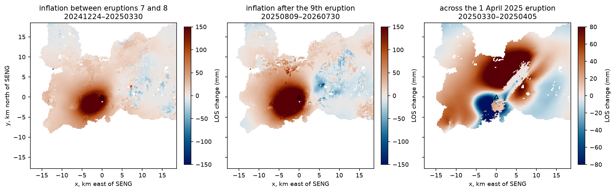

The two inflation maps show the same bulge as in Parts 1 and 2: the source has not moved. The map across the eruption is completely different. It contains the deflation of the reservoir (blue, around and south-west of SENG) and the opening of a dyke along the Sundhnúkur crater row, which pushes the ground apart and produces the red and blue lobes on either side of a north-east line. Notice that the colour scale had to be halved: within six days, the eruption reversed about a quarter of the uplift that had accumulated over the previous three months at SENG (−36 mm against +162 mm).

Step 5: validate with GNSS at SENG

The Nevada Geodetic Laboratory (NGL; Blewitt et al., 2018) publishes daily positions for GNSS stations SENG, in the middle of the deformation, and NYLA, 18 km to the north-west in the InSAR reference area. InSAR measures motion relative to its reference, so we compare it with SENG minus NYLA, which removes plate motion and most common-mode GNSS error.

GNSS gives three components; InSAR gives one. Project the GNSS displacement onto the LOS unit vector (E, N, U) of the InSAR pixel at SENG, read from the frame’s metadata GeoTIFFs (Part 1):

d_LOS = E·d_e + N·d_n + U·d_u

seng, ref = load_ngl("SENG"), load_ngl(REF_STATION)
rel = (seng - ref).dropna().loc[dt[0] - pd.Timedelta(days=3):dt[-1] + pd.Timedelta(days=3)]
vec = {}
for k in "ENU":
    a, t = read_window(f"{BASE}/metadata/{FRAME}.geo.{k}.tif")
    vec[k] = float(a[int((SENG[1] - t.f) / t.e), int((SENG[0] - t.c) / t.a)])
rel["LOS"] = vec["E"] * rel["E"] + vec["N"] * rel["N"] + vec["U"] * rel["U"]
g_ep = np.array([rel.loc[d - pd.Timedelta(days=1):d + pd.Timedelta(days=1), "LOS"].mean() for d in dt])
i_ep = np.array([np.nanmedian(ts[i, sr - 1:sr + 2, sc - 1:sc + 2]) for i in range(len(epochs))])

load_ngl is the same reader as in Part 1: it adds the reference values e0, n0, u0 back to the offsets and corrects the height for antenna changes. The GNSS series is averaged over three days around each Sentinel-1 date, and the InSAR series is the median of the 3 × 3 pixels (about 600 m) around the station.

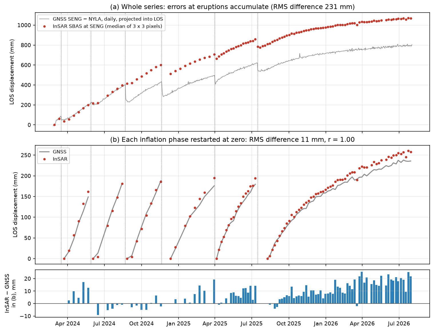
823 common daily solutions; LOS unit vector at SENG: E -0.555 N -0.123 U +0.823
InSAR at SENG: 112 epochs; GNSS on 109 of them
total LOS change 20240228-20260730: InSAR +1068 mm, GNSS +793 mm
raw InSAR - GNSS: RMS 231 mm, max 279 mm; r = 0.990
co-eruptive steps (last epoch before -> first epoch after each eruption onset):
  2024-03-16: InSAR   -26 mm, GNSS   -20 mm; 3 of 3 spanning pairs unwrapped and coherent at SENG
  2024-05-29: InSAR   +17 mm, GNSS    +2 mm; 0 of 3 spanning pairs unwrapped and coherent at SENG
  2024-08-22: InSAR   +19 mm, GNSS  -142 mm; 0 of 3 spanning pairs unwrapped and coherent at SENG
  2024-11-20: InSAR   -89 mm, GNSS  -111 mm; 1 of 1 spanning pairs unwrapped and coherent at SENG
  2025-04-01: InSAR   -41 mm, GNSS   -59 mm; 6 of 6 spanning pairs unwrapped and coherent at SENG
  2025-07-16: InSAR   -74 mm, GNSS   -43 mm; 10 of 10 spanning pairs unwrapped and coherent at SENG

The LOS vector says the ascending satellite looks from the west-south-west at about 35° from vertical: 82% of uplift and 56% of westward motion reach the LOS. Over 2.5 years, InSAR says SENG moved +1,068 mm towards the satellite, and GNSS says +793 mm. The correlation is 0.99, but the RMS difference is 231 mm. Something is badly wrong, and the co-eruptive steps show what.

Across the 22 August 2024 eruption, GNSS dropped by 142 mm, but none of the three interferograms spanning that eruption is usable at SENG: they decorrelated, or LiCSAR could not unwrap the dense co-eruptive fringes. For that pixel the network is split into “before” and “after”, and only the small regularisation term ties them together, along a straight line. The time series cannot see a step that no interferogram measures, so it simply continues the inflation trend (+19 mm). That single eruption explains 161 mm of the 275 mm discrepancy; the rest comes from the 29 May 2024 eruption (also 0 of 3 pairs), smaller differences at the other eruptions, and a slow excess of InSAR over GNSS during the inflation phases (next section). Where the spanning pairs are usable (March and November 2024, April and July 2025), the InSAR and GNSS steps agree to within 6–31 mm.

Phase by phase

The fair test of the inversion is the period where the data are complete: between eruptions. The function by_phase restarts both series at zero at the first epoch after each eruption (after the end of the three-week ninth eruption), compares them up to the last epoch before the next eruption, and fits a straight line to each phase for the rate.

starts = [0] + [epoch_after(ENDED.get(e, e)) for e in events]
ends = [epoch_before(e) for e in events] + [len(epochs) - 1]


def by_phase(i_series: np.ndarray):
    """Restart InSAR and GNSS at zero at the start of each inflation phase and compare them."""
    seg = np.full(len(epochs), -1)
    i_seg, g_seg = np.full(len(epochs), np.nan), np.full(len(epochs), np.nan)
    out = []
    for n, (a0, a1) in enumerate(zip(starts, ends)):
        k = np.arange(a0, a1 + 1)
        k = k[both[k] & np.isfinite(i_series[k])]
        if len(k) < 3:
            continue
        seg[k] = n
        i_seg[k], g_seg[k] = i_series[k] - i_series[k[0]], g_ep[k] - g_ep[k[0]]
        yrs = (dt[k] - dt[k[0]]).days / 365.25
        out.append({"from": f"{dt[k[0]]:%Y-%m-%d}", "to": f"{dt[k[-1]]:%Y-%m-%d}", "epochs": len(k),
                    "InSAR_mm": i_seg[k[-1]], "GNSS_mm": g_seg[k[-1]],
                    "InSAR_mm_per_yr": np.polyfit(yrs, i_seg[k], 1)[0],
                    "GNSS_mm_per_yr": np.polyfit(yrs, g_seg[k], 1)[0]})
    ok = np.isfinite(i_seg) & np.isfinite(g_seg)
    d = i_seg[ok] - g_seg[ok]
    return pd.DataFrame(out), seg, i_seg, g_seg, np.sqrt(np.mean(d ** 2)), np.corrcoef(i_seg[ok], g_seg[ok])[0, 1]

      from         to  epochs  InSAR_mm  GNSS_mm  InSAR_mm_per_yr  GNSS_mm_per_yr
2024-03-23 2024-05-22       6     162.0    149.0           1027.0           938.0
2024-06-03 2024-08-14       6     181.0    182.0            972.0           957.0
2024-08-26 2024-11-18       8     186.0    188.0            876.0           862.0
2024-12-12 2025-03-30       8     195.0    176.0            663.0           603.0
2025-04-05 2025-07-10      17     194.0    180.0            694.0           646.0
2025-08-09 2026-07-30      58     258.0    236.0            238.0           217.0
103 epochs in 6 inflation phases: InSAR - GNSS RMS 11.5 mm, r = 0.998
summed inflation-phase LOS uplift: InSAR +1175 mm, GNSS +1110 mm (+6%)

Now the agreement is excellent: 11.5 mm RMS over 103 epochs, with r = 0.998, for a signal of about 1.1 m. InSAR and GNSS tell the same story. In each of the first five phases, SENG rose by 150–195 mm in the LOS before the next eruption. The rate fell from about 940–1,030 mm/yr in spring 2024 to 600–700 mm/yr in 2025, and to only 217–238 mm/yr in the long phase since August 2025, which had not ended in an eruption by the end of July 2026. The slowing of the uplift is the same trend seen in the GNSS series in Part 1. It means that, after the ninth eruption, the reservoir took much longer to refill to its previous level.

Is there a phase bias?

The bottom panel shows a pattern: InSAR runs ahead of GNSS, by about 20 mm (9%) after a year in the last phase. Short-interval interferograms can contain a small systematic phase bias, often linked to changes in soil moisture and vegetation, that does not cancel when interferograms are combined and therefore accumulates in a time series built mainly from short pairs (Ansari et al., 2021). The usual test is to rebuild the series without the shortest pairs and see whether the drift changes. To make the test clean, the script averages the 3 × 3 pixels at SENG in each interferogram and solves that single averaged pixel.

obs_seng = np.array([np.nanmedian(u[sr - 1:sr + 2, sc - 1:sc + 2]) for u in unw])
for min_days in (0, 12, 18):
    keep = np.array([days(p) >= min_days for p in pairs]) & np.isfinite(obs_seng) & use_seng
    Ak = A[keep]
    rank = np.linalg.matrix_rank(Ak)
    xk = np.linalg.solve(Ak.T @ Ak + R, Ak.T @ obs_seng[keep])
    ik = np.r_[0, xk] * RAD2MM
    ik = ik - ik[k0]
    tab, *_, rms_k, r_k = by_phase(ik)

pairs >=  0 days: 355 pairs, rank 109/111; summed inflation InSAR +1148 vs GNSS +1110 mm (+3%); last phase +222 vs +217 mm/yr; RMS 4.9 mm
pairs >= 12 days: 276 pairs, rank 109/111; summed inflation InSAR +1147 vs GNSS +1110 mm (+3%); last phase +222 vs +217 mm/yr; RMS 5.0 mm
pairs >= 18 days: 172 pairs, rank 104/111; summed inflation InSAR +1193 vs GNSS +1110 mm (+7%); last phase +223 vs +217 mm/yr; RMS 12.5 mm

Two results stand out. First, solving the averaged pixel instead of taking the median of nine separately solved pixels halves the excess, from +6% to +3%, and the RMS falls to 4.9 mm: the 3 × 3 pixels have slightly different networks, and the median of their solutions is noisier. Second, dropping the 6-day pairs changes nothing, and dropping everything shorter than 18 days only makes the network weaker (rank 104 of 111) and the fit worse. A phase bias in short pairs would shrink when they are removed, so this test finds no evidence for one at SENG. The remaining 2–3% may come from the reference (InSAR’s far field and NYLA are not exactly the same “zero”), seasonal atmosphere, or the difference between a 200 m pixel and a point on a steep deformation gradient. A 3% agreement between two independent techniques over 1.1 m of motion is a good result.

Step 6: coherence loss over fresh lava

New lava destroys coherence completely: the ground surface that reflected the radar signal has been buried. Strong deformation does the same in a different way, by packing fringes more densely than the pixel size can resolve. Both happen during an eruption. The script compares the full-resolution coherence of a pair just before the 29 May 2024 eruption with the shortest pair spanning it, both 12 days long, in a 13 km window around the crater row.

before = [p for p in pairs if p[9:] < LAVA_EVENT.replace("-", "")]
across = [p for p in pairs if p[:8] < LAVA_EVENT.replace("-", "") < p[9:]]
p_across = min(across, key=days)
recent = [p for p in before if days(p) == days(p_across) and (dt[idx[p_across[:8]]] - pd.Timestamp(p[:8])).days <= 36]
p_before = max(recent, key=lambda p: med_coh[pairs.index(p)])     # the most coherent recent pair of equal span

before: 20240510_20240522 median coherence 0.34; across: 20240522_20240603 0.34 (zoom 13 x 13 km around Sundhnukur)
pixels coherent before (> 0.5) but incoherent across the eruption (< 0.2): 6.4 km2
land pixels usable in < 50% of pairs: 2.0%; at SENG 90%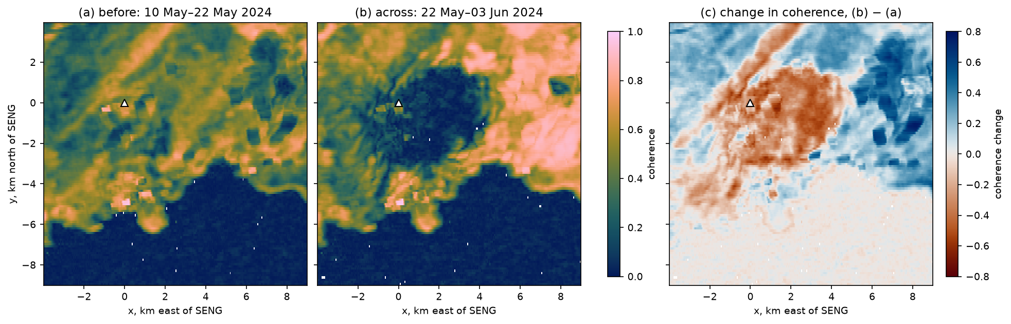

The median coherence over the window is unchanged at 0.34, because coherence improved to the north-east for reasons unrelated to the eruption (weather and ground conditions differ between the two pairs), but a patch of 6.4 km² around and east of SENG lost coherence completely. That is why none of the pairs spanning this eruption was usable at SENG in Step 5. Coherence alone cannot tell you whether a pixel decorrelated because it was buried by lava or because the deformation gradient was too steep; for that, compare with the lava outlines mapped by Icelandic institutions. After an eruption, a new lava surface becomes coherent again in later pairs, but its phase is then the motion of the cooling, contracting flow, not of the ground beneath.

Over the whole stack, only 2.0% of the land is usable in fewer than half the pairs, and SENG is usable in 90%. The losses are concentrated in time (winters and eruptions), not in space, which is exactly the situation in which an SBAS time series can look complete but be wrong at the moments that matter.

Limitations and caveats

• Co-eruptive gaps. The biggest error in this time series is not noise but missing data across two eruptions. Never interpret cumulative InSAR displacement across an event without checking that pairs spanning it were usable at that pixel.
• Atmosphere. No tropospheric correction was applied beyond the plane per interferogram. The far-field epoch-to-epoch scatter is 2.7 mm, and turbulent delay near the volcano is similar. LiCSBAS (Morishita et al., 2020) can apply GACOS weather-model corrections and temporal filtering; the inflation signal here is large enough not to need them.
• The reference. InSAR is referenced to land more than 15 km from SENG, and GNSS to NYLA. At those distances the uplift from a 4–5 km deep source is a few per cent of the peak, so both references move slightly with the volcano, though by similar amounts.
• Unwrapping. Closure finds most 2π errors, but not those in pairs that do not belong to a closed, coherent loop. Pixels with residuals above π in any pair (1.1%) deserve suspicion.
• One geometry. The time series is LOS displacement from one track. To split it into vertical and horizontal motion you need a second track over the same period (Part 1) or a source model (Part 2).
• Data volume. Multilooking to about 200 m loses detail close to the eruptive fissures. It is a deliberate choice to keep the whole stack in memory on a laptop.
• Dates. The results depend on the LiCSAR archive as accessed in October 2026. New pairs are added continually, so rerunning later with a different END will give a longer series.

Try it yourself

1. Change the coherence threshold. Rerun with MIN_COH = 0.15 and MIN_COH = 0.35. How many pairs spanning the May and August 2024 eruptions become usable at SENG, how does the whole-series RMS of 231 mm change, and how many pixels pass closure?
2. Change the network. Set MAX_DAYS = 12 to keep only 6- and 12-day pairs. Is the network still connected (rank of A), and does the phase-by-phase agreement with GNSS change? Then look at the folder listing to see whether LiCSAR offers longer pairs that could bridge the 2024 eruptions.
3. Another GNSS station. NGL also processes stations AUSV (4.3 km south of SENG, data from November 2023) and GEVK (5.5 km south-south-west, from April 2024). Change load_ngl("SENG") to the new station and SENG to its (longitude, latitude): (−22.4169, 63.8436) for AUSV or (−22.4716, 63.8354) for GEVK. Is the agreement as good closer to Grindavík and the dykes?
4. Another eruption. Set LAVA_EVENT = "2024-08-22" or "2024-11-20" and compare the area of lost coherence with the 6.4 km² of May 2024.
5. Fit a Mogi source to each phase. Save ts[j] - ts[i] for each inflation phase in the by_phase table, and fit it with the Mogi model and LOS projection from Part 2 (fixing ν = 0.25 and using the ascending unit vectors only). Does the source depth stay the same while the volume rate falls?
6. Compare with the COMET Volcano Portal. The portal publishes its own LiCSBAS time series for Reykjanes. Find the ascending frame for Svartsengi on the COMET Volcano Portal, and compare its cumulative displacement at SENG with yours. Remember that it uses a different reference.
7. The descending track. Change FRAME to 155D_02484_191814, the track number in BASE to 155, and END to 20260203. The LOS vector changes sign in the east component; does the descending time series agree with GNSS too?

Frequently asked questions

What is an InSAR time series?

An InSAR time series gives the displacement of each pixel at every acquisition date, rather than just between two dates. It is computed from many interferograms by least squares. Small baseline (SBAS) methods use a network of interferograms with short time spans; persistent scatterer (PS) methods use single, stable reflectors in full-resolution images.

How does the SBAS method work?

Each unwrapped interferogram measures the difference in displacement between its two dates. Writing that for every pair gives a linear system φ = A x, where x is the displacement at each date relative to the first. If the network of pairs is connected, the system can be solved by least squares at each pixel. Weighting by coherence and adding a small smoothness term handle missing data.

How do you compare InSAR with GNSS?

Project the GNSS east, north and up displacements into the radar line of sight using the LOS unit vector at the station, d_LOS = E·d_e + N·d_n + U·d_u. Difference the station with a GNSS station in the InSAR reference area, average a few pixels of InSAR around the station, and compare the two series on the radar acquisition dates, starting both at zero on the same date.

What is phase closure in InSAR?

For three interferograms forming a loop, such as dates 1→2, 2→3 and 1→3, the phases should satisfy φ₁₂ + φ₂₃ − φ₁₃ ≈ 0. A closure near a multiple of 2π reveals an unwrapping error. A small, non-zero closure that is not a multiple of 2π reveals a phase bias, for example from soil moisture changes.

Why does InSAR lose coherence on volcanoes?

Coherence is lost when the scattering surface changes between the two images. On volcanoes, the main causes are new lava flows and ash, snow, vegetation, and deformation so fast that the fringes are denser than the pixels. Long time intervals make all of these worse, so volcano monitoring relies on short, frequent pairs.

How fast is Svartsengi inflating?

In this time series, the SENG GNSS station rose towards the ascending Sentinel-1 satellite at 940–1,030 mm/yr in spring 2024, 600–700 mm/yr in 2025, and only 217–238 mm/yr between August 2025 and July 2026. Most of this is vertical uplift. The Icelandic Meteorological Office publishes regular updates on the uplift and the volume of magma accumulated beneath Svartsengi.

Next steps

• Part 1: mapping volcano deformation with InSAR explains fringes, LOS unit vectors and the ascending–descending decomposition used here.
• Part 2: Mogi and Okada source inversion turns a deformation map into a source depth and volume; try exercise 5 above to apply it to each inflation phase.
• For a production-quality time series with atmospheric corrections, look at LiCSBAS (Morishita et al., 2020) for LiCSAR products, or MintPy (Yunjun et al., 2019), which is used in InSAR ground subsidence in Python.

Data and licences

• COMET LiCSAR products: contain modified Copernicus Sentinel data 2024–2026, processed by COMET (LiCSAR). Open data under CC BY 4.0. Frame 016A_02504_162118, accessed from the COMET LiCSAR archive in October 2026.
• GNSS: stations SENG and NYLA, daily positions in the IGS20 frame from the Nevada Geodetic Laboratory, University of Nevada, Reno (Blewitt, G., Hammond, W. C. and Kreemer, C. (2018), “Harnessing the GPS data explosion for interdisciplinary science”, Eos 99).
• Eruption dates: Icelandic Meteorological Office news updates on the Sundhnúkur crater row (vedur.is), 2023–2026.
• References: Berardino, P., Fornaro, G., Lanari, R. and Sansosti, E. (2002), “A new algorithm for surface deformation monitoring based on small baseline differential SAR interferograms”, IEEE Transactions on Geoscience and Remote Sensing 40(11), 2375–2383; Ansari, H., De Zan, F. and Parizzi, A. (2021), “Study of systematic bias in measuring surface deformation with SAR interferometry”, IEEE Transactions on Geoscience and Remote Sensing 59(2), 1285–1301; Lazecký, M. et al. (2020), “LiCSAR: an automatic InSAR tool for measuring and monitoring tectonic and volcanic activity”, Remote Sensing 12(15), 2430; Morishita, Y. et al. (2020), “LiCSBAS: an open-source InSAR time series analysis package integrated with the LiCSAR automated Sentinel-1 InSAR processor”, Remote Sensing 12(3), 424; Yunjun, Z., Fattahi, H. and Amelung, F. (2019), “Small baseline InSAR time series analysis: unwrapping error correction and noise reduction”, Computers & Geosciences 133, 104331; Sigmundsson, F. et al. (2024), Science 383, 1228–1235.
• Colour maps: Crameri, F. (2018), Scientific colour maps (vik, batlow), via the cmcrameri package.
• Code: insar_gnss_timeseries.py, tested with Python 3.12.0, requests 2.34.2, rasterio 1.5.2, NumPy 2.5.4, pandas 3.0.6, Matplotlib 3.11.2 and cmcrameri 1.10.