InSAR volcano deformation in Python: mapping magma inflation at Svartsengi, Iceland, with Sentinel-1

Short answer: to map volcano deformation with InSAR in Python, stream unwrapped Sentinel-1 interferograms of the volcano, for example from COMET LiCSAR, which needs no login. Convert the unwrapped phase φ to line-of-sight (LOS) displacement with d = −λφ/(4π): 4.41 mm per radian, or 27.7 mm per fringe, for Sentinel-1. Mask low-coherence pixels and subtract a far-field reference area. One track gives only the LOS component. To get vertical and east–west motion, take an ascending and a descending interferogram over the same period, read the LOS unit vectors (E, N, U) for each track, and solve the two equations d = E·e + U·u at every pixel. Check the result against a GNSS station projected into the LOS.

Since November 2023 the Reykjanes Peninsula in south-west Iceland has been the best-observed volcanic system on Earth. Magma collects in a reservoir about 4–5 km beneath Svartsengi, the geothermal power station next to the Blue Lagoon. The ground above it rises by several millimetres a day. Every few months the pressure breaks the crust, magma escapes sideways in a dyke along the Sundhnúkur crater row, an eruption begins, and the ground drops. Then it starts rising again. The town of Grindavík, 4 km to the south, was evacuated when the first dyke formed on 10 November 2023.

For a student of volcano geodesy, this is an ideal natural laboratory. The signal is large (tens of centimetres), the cycle repeats, the area is mostly bare lava with good radar coherence, and a GNSS station, SENG, sits on top of the uplift. This series uses it throughout:

1. Part 1 (this tutorial): map the deformation from Sentinel-1 interferograms. Read wrapped and unwrapped phase and coherence, count fringes, and decompose ascending and descending LOS into vertical and east–west motion.
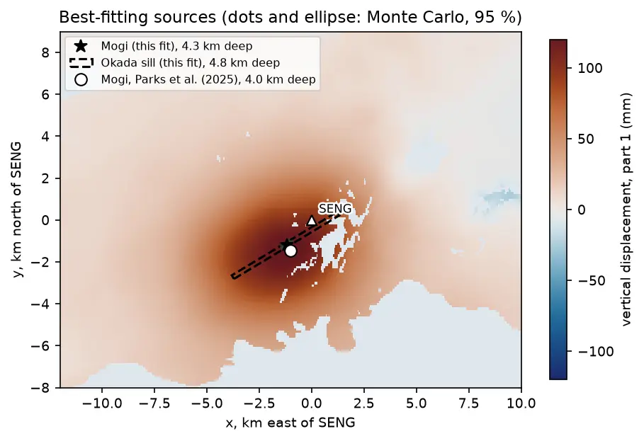
2. Part 2: model the magma source. Write Mogi point-source and Okada sill forward models in NumPy, downsample the maps from this part with a quadtree, and invert them for the depth and volume change of the reservoir, with Monte Carlo uncertainties.
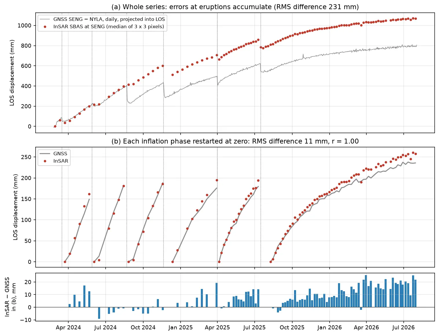
3. Part 3: build an InSAR time series of the inflation–eruption cycles from 364 interferograms, and validate it against GNSS, with a frank look at unwrapping errors, the reference point and coherence loss over fresh lava.

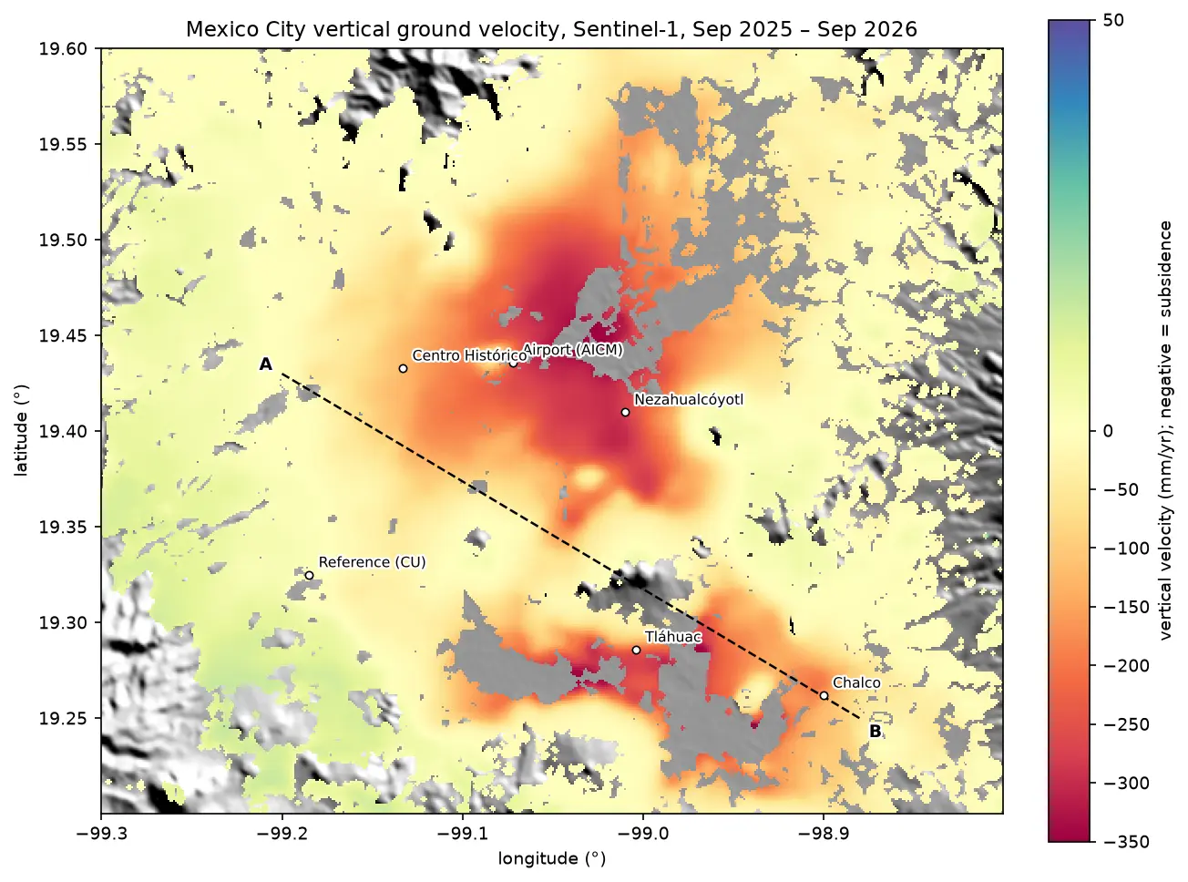
All results below are real outputs of insar_volcano_deformation.py, run on 21 October 2026 with Python 3.12, rasterio 1.5.2 and NumPy 2.5.4. If you have never seen an interferogram, InSAR ground subsidence in Python covers the basics with Mexico City, and Sentinel-1 SAR flood mapping explains radar backscatter.

The physics in four equations

Sentinel-1 is a C-band radar with a wavelength λ = 5.547 cm. An interferogram is the phase difference between two images of the same place. Once the processor has removed the effects of orbit geometry and topography, the remaining phase φ is mostly the change in the two-way path between the satellite and the ground. A ground displacement d towards the satellite shortens the path by 2d, so

φ = −4π d / λ and therefore d = −λ φ / (4π)

The sign follows the LiCSAR convention: negative unwrapped phase means motion towards the satellite. One radian is 4.41 mm, and one fringe (2π) is λ/2 = 27.7 mm.

The ground moves in three dimensions, (e, n, u) for east, north and up. The radar only measures the projection onto the line of sight. If ŝ = (E, N, U) is the unit vector from the ground to the satellite, then

d_LOS = E·e + N·n + U·u

For a satellite with heading α (the flight direction, clockwise from north) and local incidence angle θ, Sentinel-1 looks to the right, so

E = −sin θ · cos α, N = sin θ · sin α, U = cos θ

For the ascending frame over Svartsengi, α ≈ −11.7° (flying slightly west of north) and θ ≈ 35°. That gives E ≈ −0.56: the satellite is to the west of the ground, looking east. The descending frame flies south (α ≈ −168°) and looks west, so E ≈ +0.60. The north components are tiny, about −0.12 on both tracks, because both orbits are near-polar. Satellites in near-polar orbits are almost blind to north–south motion.

Finally, with an ascending LOS map d_a and a descending one d_d over the same period, and neglecting north, we have two equations in two unknowns at each pixel:

[d_a, d_d]^T = G · [e, u]^T, with G = [[E_a, U_a], [E_d, U_d]]

The solution by Cramer’s rule is e = (U_d d_a − U_a d_d) / det G and u = (E_a d_d − E_d d_a) / det G.

Step 1: find the Sentinel-1 frames over Svartsengi

LiCSAR organises its products by frame. Two frames cover Svartsengi: ascending 016A_02504_162118 (relative orbit 16) and descending 155D_02484_191814 (relative orbit 155). Each interferogram is a folder named <first date>_<second date>. We read the folder listing and the frame’s metadata.txt, which gives the heading and incidence angle.

For the decomposition we need an ascending and a descending interferogram covering roughly the same period. No single pair is ideal: 6- and 12-day pairs give too little signal, and long pairs lose coherence. So we add two consecutive 24-day pairs on each track, giving 48 days from mid-August to the end of September 2025. That is just after the ninth eruption ended on 5 August 2025, when the reservoir was refilling quickly.

LICSAR = "https://gws-access.jasmin.ac.uk/public/nceo_geohazards/LiCSAR_products.public"
TRACKS = {  # Sentinel-1 frame, and two consecutive 24-day pairs that span about 48 days
    "ascending": ("016A_02504_162118", ["20250815_20250908", "20250908_20251002"]),
    "descending": ("155D_02484_191814", ["20250813_20250906", "20250906_20250930"]),
}
BBOX = (-22.80, 63.72, -22.05, 64.05)    # lon/lat window: Reykjanes Peninsula around Svartsengi
SENG = (-22.4338, 63.8822)               # GNSS station SENG at the Svartsengi power station
REF_KM = 15                              # reference = median of land pixels > 15 km from SENG
MIN_COH = 0.3                            # ignore pixels with coherence below this in any pair
WAVELENGTH = 0.0554658                   # Sentinel-1 C-band wavelength in metres
RAD2MM = -WAVELENGTH / (4 * np.pi) * 1000  # LiCSAR convention: positive = towards the satellite


def base(frame: str) -> str:
    return f"{LICSAR}/{int(frame[:3])}/{frame}"


for track, (frame, pairs) in TRACKS.items():
    html = requests.get(f"{base(frame)}/interferograms/", timeout=60).text
    online = sorted(set(re.findall(r'href="(\d{8}_\d{8})/"', html)))
    m = dict(tok.split("=", 1) for tok in requests.get(f"{base(frame)}/metadata/metadata.txt", timeout=60)
             .text.split() if "=" in tok)
    print(f"{track:10s} {frame}: {len(online):,} interferograms online ({online[0][:8]} to {online[-1][9:]}), "
          f"heading {float(m['heading']):.1f} deg, mean incidence {float(m['avg_incidence_angle']):.1f} deg, "
          f"overpass {':'.join(m['center_time'].split(':')[:2]):>5s} UTC")

ascending  016A_02504_162118: 6,427 interferograms online (20150110 to 20260730), heading -11.7 deg, mean incidence 39.2 deg, overpass 18:59 UTC
           using 20250815_20250908 + 20250908_20251002 = 48 days
descending 155D_02484_191814: 2,685 interferograms online (20141121 to 20260203), heading -168.3 deg, mean incidence 39.2 deg, overpass  7:57 UTC
           using 20250813_20250906 + 20250906_20250930 = 48 days

The ascending frame holds more than 6,000 interferograms because COMET processes it routinely for this eruption crisis. The descending archive stopped in February 2026, which is one reason Part 3 uses the ascending track.

Step 2: stream only the window you need

LiCSAR GeoTIFFs cover a whole frame, about 250 × 250 km. GDAL can read a remote GeoTIFF with HTTP range requests, so we fetch only the rows that cover our 0.75° × 0.33° window and cache them as compressed NumPy files. Reruns are then instant.

def read_window(url: str):
    """Read only the rows of a remote LiCSAR GeoTIFF that cover BBOX (HTTP range requests)."""
    with rasterio.open(url) as src:
        win = from_bounds(*BBOX, src.transform).round_offsets().round_lengths()
        return src.read(1, window=win).astype("float32"), src.window_transform(win)


def cached(name: str, url: str):
    """Read a window once and keep it in data/ so that reruns are instant."""
    f = DATA / f"{name}.npz"
    if not f.exists():
        a, t = read_window(url)
        np.savez_compressed(f, a=a, t=np.array(t)[:6])
    z = np.load(f)
    return z["a"], rasterio.Affine(*z["t"])

Step 3: wrapped phase, unwrapped phase and coherence

To see clear fringes we need a long pair, with lots of deformation. The ascending pair 8 September 2025 to 5 June 2026 spans 270 days of steady inflation with no eruption in between. We read three files for it: .geo.diff_pha.tif (wrapped phase, −π to π), .geo.unw.tif (unwrapped phase in radians, where 0 means not unwrapped) and .geo.cc.tif (coherence, stored as 0–255).

An interferogram is relative: it has an unknown constant offset. We remove it by subtracting the median of all land pixels more than 15 km from SENG, which we treat as stable.

url = f"{base(frame)}/interferograms/{SHOWCASE}/{SHOWCASE}"
wrapped, transform = cached(f"asc_{SHOWCASE}_pha", f"{url}.geo.diff_pha.tif")
unw, _ = cached(f"asc_{SHOWCASE}_unw", f"{url}.geo.unw.tif")
coh, _ = cached(f"asc_{SHOWCASE}_cc", f"{url}.geo.cc.tif")
land = unw != 0                                          # 0 = sea or not unwrapped
unw[~land], wrapped[~land] = np.nan, np.nan
coh = np.where(land, coh / 255, np.nan)                  # LiCSAR stores coherence as 0-255
# ... lon/lat grids and the distance of every pixel from SENG ...
far = land & (dist_km > REF_KM)
unw_ref = unw - np.nanmedian(unw[far])
at_seng = np.nanmedian(unw_ref[sr - 1:sr + 2, sc - 1:sc + 2])
print(f"unwrapped phase at SENG relative to the far field: {at_seng:.2f} rad = {at_seng / (2 * np.pi):.2f} "
      f"fringes = {at_seng * RAD2MM:+.1f} mm LOS (one fringe = {abs(2 * np.pi * RAD2MM):.1f} mm)")

pair 20250908_20260605 (270 days), window 330 x 750 pixels of 0.001 deg (about 49 m x 111 m)
land pixels 51%; median coherence on land 0.40; far-field reference pixels (> 15 km from SENG): 39,223
unwrapped phase at SENG relative to the far field: -40.57 rad = -6.46 fringes = +179.1 mm LOS (one fringe = 27.7 mm)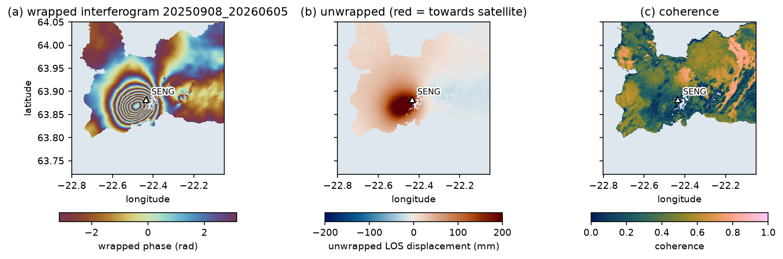

The bullseye of concentric fringes in (a) is the classic signature of a pressurised magma body. It is centred about 2 km west-south-west of SENG, not under the eruption sites on the Sundhnúkur crater row 3–4 km to the east. Magma is stored under Svartsengi and travels sideways to erupt. The wrapped phase decreases towards the centre (the colours cycle in the negative direction), which in the LiCSAR convention is motion towards the satellite: uplift.

The coherence map (c) has a median of 0.40, low for an arid site but reasonable for a 270-day pair in Iceland that includes a winter of snow. LiCSAR unwrapped almost everything except a few patches east of SENG, mostly on the newest lava flows. Part 3 looks at that coherence loss in detail.

Step 4: count the fringes

Counting fringes is the oldest way to read an interferogram, and it is a good check on the unwrapping. Along a profile from the far field to the peak, every jump of 2π in the wrapped phase is one fringe. The unwrapped phase should change by the same number of cycles.

pr = int((~transform * (0, PROFILE_LAT))[1])
row_w = np.angle(np.nanmean(np.exp(1j * wrapped[pr - 3:pr + 4]), axis=0))  # circular mean of 7 rows
row_u = np.nanmedian(unw_ref[pr - 3:pr + 4], axis=0)
ok = (lon > PROFILE_LON[0]) & (lon < PROFILE_LON[1]) & np.isfinite(row_w) & np.isfinite(row_u)
ok &= lon <= lon[ok][np.argmax(np.abs(row_u[ok]))]      # stop at the peak of the LOS signal
jumps = np.abs(np.diff(row_w[ok])) > np.pi
cycles = (row_u[ok][-1] - row_u[ok][0]) / (2 * np.pi)

profile along 63.868 N from -22.725 to the LOS peak at -22.479 E: 8 wrapped-phase jumps counted; unwrapped phase changes by -8.44 cycles = 234 mm

Averaging phase needs care. You cannot take the arithmetic mean of wrapped angles: the mean of +3.1 and −3.1 rad is 0, but both are almost π. The code averages the unit phasors exp(iφ) and takes the angle of the result, which is the circular mean.

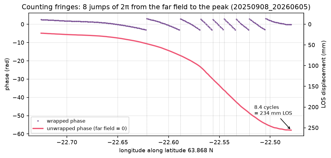
The two agree: 8 complete fringes, and 8.44 cycles of unwrapped phase, because the profile does not start or end exactly on a fringe boundary. Note also that the far field is not exactly zero on this profile: the reference is the median of the whole far-field area, and the western end sits on the edge of the deformation.

Is +179 mm at SENG right? The GNSS station measured its own motion over the same 270 days (Step 7). Projected into the ascending LOS, it predicts +184.0 mm, or 6.64 fringes, against 6.46 from InSAR. That is a difference of 5 mm, or less than a fifth of a fringe, after nine months.

Step 5: build ascending and descending LOS maps

For the decomposition we now switch to the four 24-day pairs. Each is masked where its coherence is below 0.3 or it was not unwrapped. Then a plane, a + b·lon + c·lat, is fitted to the far-field pixels and subtracted. This removes the constant offset and also any long-wavelength ramp from orbit errors, the ionosphere or large-scale tropospheric gradients. The two pairs on each track are added.

def deramp(u: np.ndarray, use: np.ndarray, LON: np.ndarray, LAT: np.ndarray):
    """Fit a + b*lon + c*lat to the far-field pixels and subtract it (orbit/ionosphere/long-wave tropo)."""
    A = np.column_stack([np.ones(use.sum()), LON[use] - LON.mean(), LAT[use] - LAT.mean()])
    coef = np.linalg.lstsq(A, u[use], rcond=None)[0]
    return u - (coef[0] + coef[1] * (LON - LON.mean()) + coef[2] * (LAT - LAT.mean())), coef


for track, (frame, pairs) in TRACKS.items():
    tag = "asc" if track == "ascending" else "desc"
    total, good = np.zeros((H, W), "float32"), np.ones((H, W), bool)
    for p in pairs:
        u, t = cached(f"{tag}_{p}_unw", f"{base(frame)}/interferograms/{p}/{p}.geo.unw.tif")
        c, _ = cached(f"{tag}_{p}_cc", f"{base(frame)}/interferograms/{p}/{p}.geo.cc.tif")
        ok_p = (u != 0) & (c / 255 >= MIN_COH) & land
        good &= ok_p
        u = np.where(ok_p, u, np.nan)
        u, coef = deramp(u, far & ok_p, LON, LAT)        # re-reference AND remove a plane, every pair
        total += np.nan_to_num(u) * RAD2MM
    los[track] = np.where(good, total, np.nan)
    vec[track] = np.stack([cached(f"{tag}_{k}", f"{base(frame)}/metadata/{frame}.geo.{k}.tif")[0]
                           for k in "ENU"])

ascending  20250815_20250908: median coherence 0.89, usable 98% of land, ramp removed 15 mm W-E and 20 mm S-N across the window
ascending  20250908_20251002: median coherence 0.87, usable 98% of land, ramp removed 10 mm W-E and 9 mm S-N across the window
ascending  20250815-20251002: max +109.0 mm, SENG +77.8 mm, far-field scatter (std) 4.8 mm, usable 98% of land
descending 20250813_20250906: median coherence 0.85, usable 97% of land, ramp removed 92 mm W-E and 14 mm S-N across the window
descending 20250906_20250930: median coherence 0.83, usable 97% of land, ramp removed 12 mm W-E and 3 mm S-N across the window
descending 20250813-20250930: max +104.0 mm, SENG +89.8 mm, far-field scatter (std) 4.2 mm, usable 97% of land

Snow-free late-summer pairs have coherence above 0.8, so 97–98% of the land is usable. Most ramps are 10–20 mm across the window, but the first descending pair had a 92 mm west–east ramp: an ionospheric or tropospheric gradient that would otherwise have tilted the whole map. After deramping, the far-field scatter is 4–5 mm, which is the noise level of these maps.

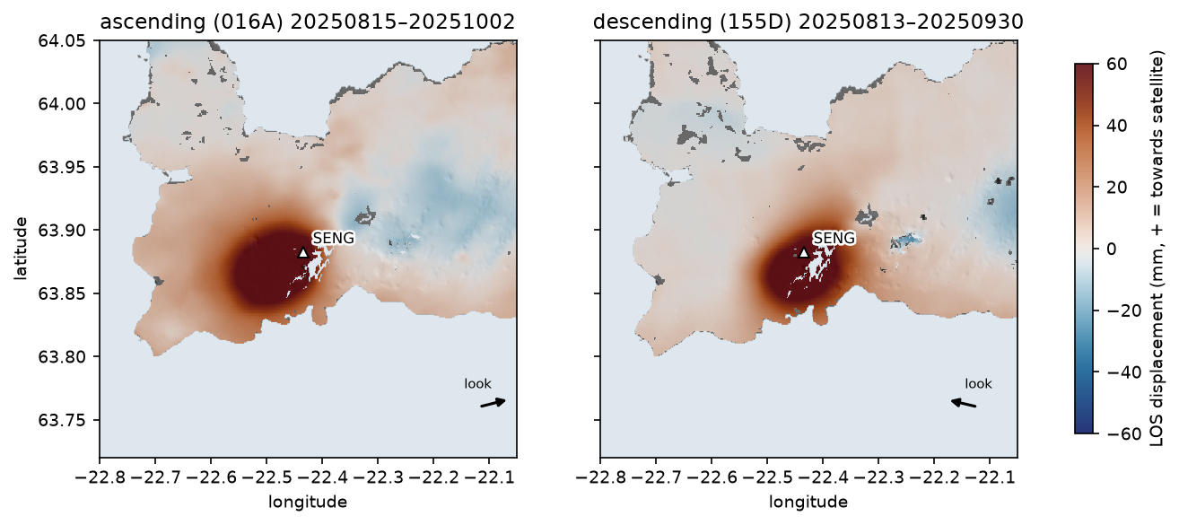
The two maps are similar, because the motion is mostly vertical, but not identical. The ascending bullseye is centred slightly further west. An inflating source pushes the ground outwards as well as up. West of the centre the ground moves west, towards the ascending satellite, which adds to the LOS signal; east of the centre the ground moves east, away from it. The descending track sees the mirror image. That asymmetry is exactly what the decomposition uses.

The LOS unit vectors come from the frame’s E, N and U GeoTIFFs. At SENG:

ascending  E -0.555  N -0.123  U +0.823  -> incidence 34.7 deg, look azimuth 77.5 deg
descending E +0.597  N -0.123  U +0.793  -> incidence 37.5 deg, look azimuth 281.7 deg

These match the formulas above: θ = arccos U, and the horizontal look direction (from the satellite towards the ground) is about 78° (east-north-east) on the ascending track and 282° (west-north-west) on the descending one. The incidence angle varies across each frame, from about 30° to 46°, so always use the per-pixel files rather than one mean angle. The metadata’s mean of 39.2° is not the value at SENG.

Step 6: decompose into vertical and east–west motion

With two LOS maps and two unknowns per pixel, the solution is Cramer’s rule, vectorised over the whole grid:

# d_asc = E_a*e + N_a*n + U_a*u and d_desc = E_d*e + N_d*n + U_d*u. Two equations, three unknowns:
# north is dropped because both near-polar orbits are almost blind to it (N is about +/-0.1).
Ea, Na, Ua = vec["ascending"]
Ed, Nd, Ud = vec["descending"]
det = Ea * Ud - Ed * Ua
d_a, d_d = los["ascending"], los["descending"]
east = (Ud * d_a - Ua * d_d) / det
up = (Ea * d_d - Ed * d_a) / det
G = np.array([[Ea[sr, sc], Ua[sr, sc]], [Ed[sr, sc], Ud[sr, sc]]])
cov = np.linalg.inv(G.T @ G)
print(f"noise amplification for 1 mm LOS noise: east {np.sqrt(cov[0, 0]):.2f} mm, up {np.sqrt(cov[1, 1]):.2f} mm")

design matrix at SENG [[E_a U_a] [E_d U_d]] = [[-0.555, 0.823], [0.597, 0.793]], condition number 1.40
noise amplification for 1 mm LOS noise: east 1.23 mm, up 0.88 mm
maximum uplift 121.5 mm at -22.459 E, 63.868 N; east-west range -44.0 to +34.8 mm (1st-99th pct)
at SENG: up +103.5 mm, east +12.9 mm
area with > 20 mm uplift: 106 km2

How well posed is this? If each LOS map has independent noise of standard deviation σ, the covariance of (e, u) is σ²(GᵀG)⁻¹. Its diagonal gives the noise amplification: 1 mm of LOS noise becomes 1.23 mm in east and 0.88 mm in up. The condition number, 1.40, is close to the ideal of 1, because the two tracks look from nearly opposite sides. The vertical component is better constrained than the horizontal one, because both LOS vectors are steep (U ≈ 0.8).

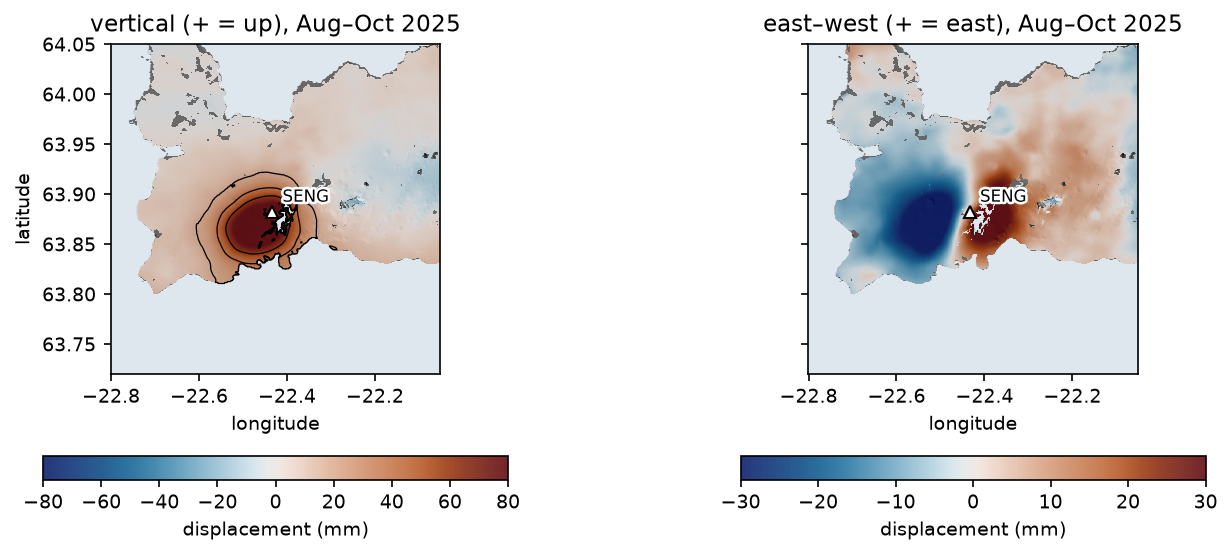
This is the textbook pattern of an inflating magma body. Vertical motion peaks over the source; horizontal motion is zero above it and points outwards on either side, peaking on the flanks. The horizontal pattern is also a quick depth gauge, as Part 2 shows: for a point source, the horizontal displacement peaks at a distance of about 0.7 times the depth from the centre.

Step 7: check against GNSS

GNSS gives 3D positions every day at one point, which makes it the natural check on InSAR. NGL publishes daily east, north and up positions for SENG in a plain-text .tenv3 file. Two details matter. First, the east, north and up columns are offsets from reference values e0, n0 and u0, which change occasionally, so add them back. Second, NGL reports the antenna height in a separate ant column, which jumps when the antenna is changed; add it to up to remove those artificial steps.

To compare with InSAR, take the change in position between the two dates (averaged over ±1 day) and project it into the LOS with the same unit vector:

txt = requests.get(f"{NGL}/SENG.tenv3", timeout=60).text
g = pd.read_csv(io.StringIO(txt), sep=r"\s+")
g.columns = [c.strip("_").split("(")[0] for c in g.columns]
g["date"] = pd.to_datetime(g["YYMMMDD"], format="%y%b%d")
g = g.set_index("date")
g["E"] = (g["e0"] + g["east"]) * 1000                    # mm; e0/n0/u0 change when the reference does
g["N"] = (g["n0"] + g["north"]) * 1000
g["U"] = (g["u0"] + g["up"] + g["ant"]) * 1000           # add the antenna height back (0 / 0.5 m steps)


def gnss_at(day: str) -> pd.Series:
    t = pd.Timestamp(day)
    return g.loc[t - pd.Timedelta(days=1):t + pd.Timedelta(days=1), ["E", "N", "U"]].mean()


for track in TRACKS:
    d0, d1 = dates[track]
    dg = gnss_at(d1) - gnss_at(d0)
    e, n, u = vec[track][:, sr, sc]
    g_los = e * dg["E"] + n * dg["N"] + u * dg["U"]

3,288 daily solutions 2015-06-26 to 2026-09-26; median sigma E/N/U 0.8/1.1/3.6 mm
ascending  20250815-20251002: GNSS dE +12.1 dN +30.3 dU +112.3 mm -> LOS +81.9 mm; InSAR +77.8 mm; difference -4.1 mm
descending 20250813-20250930: GNSS dE +14.6 dN +33.3 dU +110.6 mm -> LOS +92.3 mm; InSAR +89.8 mm; difference -2.5 mm
showcase pair 20250908_20260605: GNSS predicts +184.0 mm LOS = 6.64 fringes at SENG; the unwrapped interferogram gives +179.1 mm = 6.46
decomposed vs GNSS (14 Aug-1 Oct 2025): up +103.5 vs +108.4 mm, east +12.9 vs +11.9 mm
           InSAR_mm  GNSS_mm
component
asc. LOS       77.8     81.9
desc. LOS      89.8     92.3
vertical      103.5    108.4
east           12.9     11.9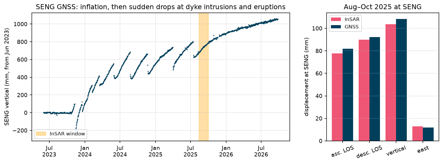

InSAR and GNSS agree to within 2.5–4.1 mm in LOS and 4.9 mm in the vertical, all within the 4–5 mm far-field noise. InSAR is slightly low in every LOS comparison. A plausible reason is spatial averaging: a 3 × 3 window of 49 × 111 m pixels averages over a few hundred metres on the side of a steep bulge, while GNSS measures one point. Atmospheric noise and residual ramps are the other candidates.

The GNSS time series also shows why the series has three parts. The sawtooth of inflation, eruption and renewed inflation is what Part 3 recovers from InSAR alone. The fact that the uplift rate in 2025–2026 is lower than in 2024 is one of the key questions Icelandic scientists have been monitoring: whether the inflow of magma from depth is slowing.

How much magma is that? A first look

A simple calculation links these numbers to a volume. For a point pressure source in an elastic half-space (the Mogi model in Part 2), the maximum uplift u_max above a source at depth d with volume change ΔV is

u_max = (1 − ν) ΔV / (π d²)

With Poisson’s ratio ν = 0.25, u_max = 0.12 m and d = 4 km, ΔV ≈ 0.12 × π × 4000² / 0.75 ≈ 8 million m³ in 48 days, or about 2 m³ per second. The Icelandic Meteorological Office reported that about 27.5 million m³ of magma had accumulated beneath Svartsengi from mid-July 2025 to early June 2026. Part 2 turns this back-of-the-envelope estimate into a proper inversion, with uncertainties.

Limitations and caveats

• North is ignored. With only two near-polar tracks, north–south motion is almost invisible. GNSS shows SENG moved 30–33 mm north in this window, and with N ≈ −0.12 on both tracks that contributes about −4 mm to each LOS value. Dropping it biases the vertical slightly. The proper fix is a third look direction, such as azimuth offsets or another satellite, or a model, as in Part 2.
• Different dates. The ascending and descending windows differ by up to two days at each end. At about 2 mm a day of uplift, this matters at the few-millimetre level. Interpolate both tracks to common dates with a time series (Part 3) for a cleaner decomposition.
• Relative measurement. Everything is relative to the far field, which we assume is stable. On the Reykjanes Peninsula the plate boundary itself moves by about 2 cm a year, and the far field partly overlaps with deformation from the wider system. The deramping plane absorbs some of the real signal on such a large deformation field.
• Atmosphere. The far-field scatter of 4–5 mm is mostly tropospheric. Iceland’s maritime climate makes it worse in winter. Single-pair maps should be read with that noise level in mind.
• Unwrapping. LiCSAR unwrapped these pairs cleanly, but long pairs with dense fringes and low coherence can contain errors of exactly one fringe (27.7 mm). Counting fringes, as in Step 4, and comparing with GNSS are good checks. Part 3 uses phase closure to find them systematically.
• Resolution. LiCSAR products are multilooked to about 0.001° (49 × 111 m here). That is fine for a volcano-wide signal, but not for individual fissures, which need full-resolution processing.

Try it yourself

Each exercise needs only a change to the constants at the top of the script, or a few lines of code.

1. A different showcase pair. Change SHOWCASE to a pair that spans an eruption, such as 20250318_20250411 (across the 1 April 2025 eruption). Look at the wrapped phase: what does the dyke do to the fringes, and does the GNSS fringe count still agree?
2. The reference area. Change REF_KM from 15 to 8 or 25 km. How much does the displacement at SENG change, and why? What does that tell you about the extent of the deformation field?
3. The coherence threshold. Set MIN_COH to 0.1 and 0.6. How does the usable area change, and is the GNSS agreement better or worse?
4. Keep north. GNSS gives dN at SENG. Subtract N * dN from each LOS value at SENG before the decomposition. How much does the vertical change?
5. Another period. Choose two consecutive 12-day pairs on each track from a different month, from the folder listings printed in Step 1, and repeat the decomposition. Does the uplift rate in millimetres a day agree with the GNSS curve in the figure above?
6. Your own volcano. Find the frames for another volcano on the COMET Volcano Portal, for example Campi Flegrei in Italy, change TRACKS, BBOX and the GNSS station, and rerun.

Frequently asked questions

How does InSAR measure volcano deformation?

InSAR compares the phase of two radar images of a volcano taken at different times. When magma accumulates, the ground above it rises and moves outwards, changing its distance to the satellite. Each change of half a radar wavelength, 27.7 mm for Sentinel-1, produces one fringe in the interferogram, so the concentric fringes around an inflating volcano can be counted, or unwrapped, to give millimetres of motion over hundreds of square kilometres.

What is a fringe in an interferogram?

A fringe is one full cycle of colour, from −π to π, in a wrapped interferogram. It represents half a radar wavelength of change in the distance to the satellite: 27.7 mm for C-band Sentinel-1, about 15 mm for X-band and about 120 mm for L-band. Counting fringes from a stable area to the centre of a bullseye gives the total line-of-sight displacement to within one fringe.

Why do I need ascending and descending InSAR?

A single InSAR track measures only the component of motion along its line of sight, which mixes vertical and horizontal motion. Ascending and descending passes look at the ground from opposite sides, east and west, so combining them separates vertical from east–west motion. North–south motion remains poorly resolved because both orbits are near-polar.

What is the line-of-sight unit vector?

It is the unit vector pointing from a ground pixel to the satellite, given as east, north and up components. LOS displacement is the dot product of this vector with the ground displacement. For Sentinel-1 the vertical component is about 0.75–0.85, and the east component is about ±0.55–0.65, depending on the track and the position in the swath.

Is Sentinel-1 InSAR data free for volcano monitoring?

Yes. Sentinel-1 data are free under the Copernicus licence. COMET LiCSAR publishes processed interferograms openly for many volcanic frames, and the COMET Volcano Portal indexes them by volcano. GNSS time series from the Nevada Geodetic Laboratory are also free. None of the data in this tutorial needs an account.

What is happening at Svartsengi in Iceland?

Since late 2023, magma has been accumulating in a reservoir about 4–5 km beneath Svartsengi on the Reykjanes Peninsula. It has drained repeatedly into dykes and fissure eruptions along the Sundhnúkur crater row, with nine eruptions between December 2023 and August 2025. The ground rises between eruptions and drops when magma leaves. The Icelandic Meteorological Office monitors it with GNSS, InSAR and seismometers.

Next steps

• Part 2: Mogi and Okada inversion in Python. Turn the vertical and LOS maps from this part into a source depth and volume change, with uncertainties. It reads data/svartsengi_los_2025.npz, which this script writes.
• Part 3: InSAR time series validated with GNSS. Follow the inflation–eruption cycles through 364 interferograms from 2024 to 2026.
• See a slower, steadier deformation signal in InSAR ground subsidence in Python, with an SBAS time series and MintPy.
• Use the same satellite’s backscatter, rather than its phase, to map water in Sentinel-1 SAR flood mapping in Python.

Data and licences

• COMET LiCSAR products: contain modified Copernicus Sentinel data 2025–2026, processed by COMET (LiCSAR). Open data under CC BY 4.0. Frames 016A_02504_162118 and 155D_02484_191814, accessed from the COMET LiCSAR archive in October 2026.
• GNSS: station SENG daily positions in the IGS20 frame from the Nevada Geodetic Laboratory, University of Nevada, Reno (Blewitt, G., Hammond, W. C. and Kreemer, C. (2018), “Harnessing the GPS data explosion for interdisciplinary science”, Eos 99).
• References: Lazecký, M. et al. (2020), “LiCSAR: an automatic InSAR tool for measuring and monitoring tectonic and volcanic activity”, Remote Sensing 12(15), 2430; Mogi, K. (1958), Bulletin of the Earthquake Research Institute 36, 99–134; Sigmundsson, F. et al. (2024), “Fracturing and tectonic stress drive ultrarapid magma flow into dikes”, Science 383, 1228–1235; Parks, M. et al. (2025), Earth and Planetary Science Letters 658, 119324, doi:10.1016/j.epsl.2025.119324; Icelandic Meteorological Office news updates on the Sundhnúkur crater row (vedur.is), 2025–2026.
• Colour maps: Crameri, F. (2018), Scientific colour maps (romaO, vik, batlow), via the cmcrameri package.
• Code: insar_volcano_deformation.py, tested with Python 3.12.0, requests 2.34.2, rasterio 1.5.2, NumPy 2.5.4, pandas 3.0.6, Matplotlib 3.11.2 and cmcrameri 1.10.