Mogi model inversion in Python: magma depth and volume from InSAR at Svartsengi, Iceland

Short answer: to invert InSAR for a Mogi source in Python, write the Mogi forward model: the surface displacement of a point pressure source at (x₀, y₀, d) with volume change ΔV is u = (1 − ν) ΔV / π · (x − x₀, y − y₀, d) / R³, where R is the distance to the source. Project it into the line of sight with the LOS unit vector, d_LOS = E·u_e + N·u_n + U·u_z. Downsample the InSAR map to a few hundred points with a quadtree, add an offset and ramp per track, and minimise the weighted misfit with scipy.optimize.least_squares. Weight with the inverse of a spatially correlated noise covariance, estimated from the residuals. For uncertainties, add correlated noise to the data and refit many times (Monte Carlo).

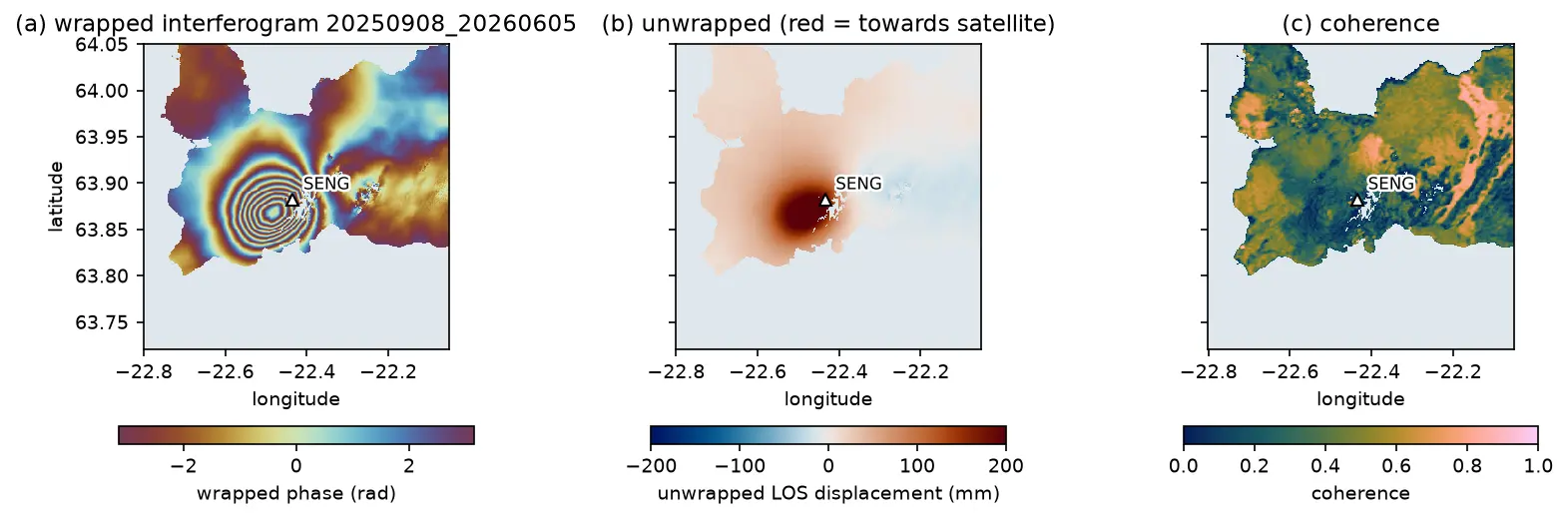
In Part 1 we mapped 48 days of uplift at Svartsengi on Iceland’s Reykjanes Peninsula from ascending and descending Sentinel-1 interferograms. The ground rose by up to 121.5 mm between mid-August and the end of September 2025, in a near-circular bulge 2 km west-south-west of the SENG GNSS station. The question for a volcanologist is: what is under there? How deep is the magma, and how much has arrived?

That is an inverse problem. We cannot see the magma, but we can calculate the surface displacement that a given source would cause (the forward model), and search for the source that best explains the data. In this tutorial you will:

1. implement the Mogi point source and the full Okada (1985) rectangular dislocation in NumPy, and check Okada against the paper’s own test values;
2. reduce 245,000 InSAR pixels to 1,349 points with a quadtree;
3. fit both models to ascending and descending data together by non-linear least squares;
4. estimate the spatially correlated noise of the data and use it to weight the inversion;
5. get uncertainties and trade-offs with a Monte Carlo of correlated noise;
6. compare the results, honestly, with published source models.

All results are real outputs of mogi_okada_inversion.py, run on 21 October 2026 with Python 3.12, NumPy 2.5.4 and SciPy 1.18.1.

Forward model 1: the Mogi point source

Kiyoo Mogi (1958) used the solution for a small spherical cavity under pressure in an elastic half-space to explain the deformation of Sakurajima and other Japanese volcanoes. For a source at horizontal position (x₀, y₀) and depth d, a surface point at horizontal distance r from the source is at distance R = √(r² + d²), and it moves by

u_r = (1 − ν) ΔV / π · r / R³, u_z = (1 − ν) ΔV / π · d / R³

where ΔV is the volume change of the source and ν is Poisson’s ratio (0.25 for a Poisson solid, λ = μ). Four properties of these equations are worth remembering:

• The shape depends only on depth. ΔV only scales the pattern. Uplift falls to half its peak value at r ≈ 0.77d, so the width of the bulge measures the depth.
• The peak horizontal displacement is at r = d/√2 ≈ 0.71d, and it is 0.38 times the peak uplift.
• Depth and volume trade off. The peak uplift is (1 − ν)ΔV/(πd²). A deeper source with more volume produces almost the same peak, so only the shape separates them.
• The shear modulus has disappeared. Written in terms of ΔV, the displacement does not depend on rigidity. Written in terms of pressure change ΔP, it would: ΔV = πa³ΔP/μ for a sphere of radius a. That is why geodesists report ΔV, not ΔP.

In NumPy the model is three lines:

NU = 0.25                                  # Poisson's ratio (lambda = mu)


def mogi(x, y, x0, y0, depth, dV, nu=NU):
    """Mogi (1958) point pressure source in an elastic half-space.
    x, y, x0, y0, depth in metres; dV = volume change of the source in m3. Returns (ue, un, uz) in metres."""
    dx, dy = x - x0, y - y0
    R3 = (dx ** 2 + dy ** 2 + depth ** 2) ** 1.5
    C = (1 - nu) * dV / np.pi
    return C * dx / R3, C * dy / R3, C * depth / R3

Forward model 2: the Okada rectangular dislocation

A point source is a sphere; magma reservoirs are often sills, flat lenses that spread horizontally. Yoshimitsu Okada (1985) published closed-form expressions for the surface displacement caused by a rectangular dislocation of length L and width W, at any dip, with strike-slip (U₁), dip-slip (U₂) or tensile opening (U₃). Tensile opening on a horizontal rectangle (dip 0°) is a sill; on a vertical one (dip 90°) it is a dyke. The same code models earthquakes.

The expressions are long, about forty terms, so the full function is in the script rather than here. They are written in Chinnery’s notation: a function f(ξ, η) is evaluated at the four corners of the rectangle and combined as

u = f(x, p) − f(x, p − W) − f(x − L, p) + f(x − L, p − W), with p = y cos δ + d sin δ

where δ is the dip and d the depth of the bottom edge. A second function, okada_rect, rotates and shifts map coordinates into Okada’s fault frame, so a sill is described by its centre, depth, length, width, strike and opening.

Transcribing forty terms is error-prone, so test it. Okada’s Table 2 lists the displacement at x = 2, y = 3 for a fault at d = 4, dip 70°, L = 3, W = 2, for unit slip of each type. The script compares all nine numbers, and stops if any differs by more than 0.2%:

okada_table2 = {"strike-slip": (-8.689e-3, -4.298e-3, -2.747e-3),
                "dip-slip": (-4.682e-3, -3.527e-2, -3.564e-2),
                "tensile": (-2.660e-4, 1.056e-2, 3.214e-3)}
for (name, ref), kw in zip(okada_table2.items(), [{"U1": 1}, {"U2": 1}, {"U3": 1}]):
    got = okada85(np.array(2.0), np.array(3.0), 4.0, 70.0, 3.0, 2.0, **kw)
    assert np.allclose(got, ref, rtol=2e-3, atol=0), "Okada implementation does not match Okada (1985) Table 2"
# A small sill should behave like a point tensile crack: uz = 3 dV d^3 / (2 pi R^5) (Okada 1985, point source)
r = np.array([0.0, 2e3, 4e3, 8e3])
dV_test = 100.0 * 100.0 * 1.0
crack = 3 * dV_test * 4e3 ** 3 / (2 * np.pi * (r ** 2 + 4e3 ** 2) ** 2.5)
sill_small = okada_rect(r, 0 * r, 0, 0, 4e3, 100.0, 100.0, 0, 0, 1.0)[2]
mogi_same = mogi(r, 0 * r, 0, 0, 4e3, dV_test)[2]

strike-slip  ux -8.689e-03 uy -4.298e-03 uz -2.747e-03 | published -8.689e-03 -4.298e-03 -2.747e-03 | max diff 4.2e-07
dip-slip     ux -4.682e-03 uy -3.527e-02 uz -3.564e-02 | published -4.682e-03 -3.527e-02 -3.564e-02 | max diff 2.7e-06
tensile      ux -2.660e-04 uy +1.056e-02 uz +3.214e-03 | published -2.660e-04 +1.056e-02 +3.214e-03 | max diff 4.1e-06
100 m x 100 m sill, 1 m opening, 4 km deep; uz in micrometres at r = 0, 2, 4, 8 km:
  Okada [298.338 170.812  52.758   5.339] | point crack formula [298.416 170.823  52.753   5.338] | Mogi, same volume [149.208 106.764  52.753  13.346]
  above the source a sill lifts the surface 2.00x more than a Mogi source of the same volume change

All nine values match to the four significant figures printed in the paper. The second test is physically interesting. A tiny sill reproduces the analytical point-crack formula u_z = 3ΔV d³ / (2πR⁵), and compared with a Mogi source of the same volume it lifts the surface twice as much directly above, but less at a distance: the sill’s pattern is narrower. A sphere spends part of its volume change pushing the rock sideways; a horizontal crack pushes almost all of it upwards. This factor of 2 will reappear when we compare the volumes from the two models.

Step 1: downsample with a quadtree

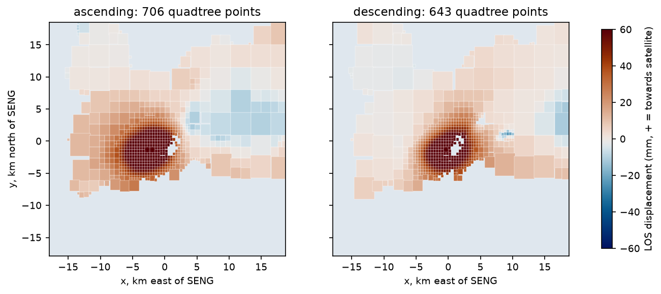
The two LOS maps have 245,462 pixels between them. Neighbouring pixels carry almost the same information, because the deformation is smooth and the noise is spatially correlated, and a full covariance matrix for that many points would need 480 GB. So we reduce the data. A quadtree splits the map into blocks and keeps splitting any block whose standard deviation exceeds a threshold (here 2.5 mm). Smooth far-field areas end up as a few big blocks; the steep flanks of the bulge get many small ones.

def quadtree(data, max_std=2.5, min_px=4, start=32, min_valid=0.5):
    """Split blocks while the LOS inside them varies more than max_std (mm). Returns leaf rows/cols/values."""
    leaves = []

    def split(r0, c0, h, w):
        blk = data[r0:r0 + h, c0:c0 + w]
        valid = np.isfinite(blk)
        if valid.mean() < min_valid:
            if h > min_px:                              # coastline: try smaller blocks
                for dr, dc in [(0, 0), (0, w // 2), (h // 2, 0), (h // 2, w // 2)]:
                    split(r0 + dr, c0 + dc, h // 2 if dr == 0 else h - h // 2, w // 2 if dc == 0 else w - w // 2)
            return
        if np.nanstd(blk) > max_std and h > min_px:
            for dr, dc in [(0, 0), (0, w // 2), (h // 2, 0), (h // 2, w // 2)]:
                split(r0 + dr, c0 + dc, h // 2 if dr == 0 else h - h // 2, w // 2 if dc == 0 else w - w // 2)
            return
        rr, cc = np.nonzero(valid)
        leaves.append((r0 + rr.mean(), c0 + cc.mean(), np.nanmean(blk), h, w))

    H, Wd = data.shape
    bh, bw = start, start * 2                           # pixels are ~49 m x 111 m: 2:1 keeps blocks square
    for r0 in range(0, H, bh):
        for c0 in range(0, Wd, bw):
            split(r0, c0, min(bh, H - r0), min(bw, Wd - c0))
    return np.array(leaves)

ascending  123,486 pixels -> 706 quadtree points (block sizes 4-32 rows)
descending 121,976 pixels -> 643 quadtree points (block sizes 4-32 rows)

Each point keeps the mean LOS value of its block, the position of the centroid of its valid pixels, and the LOS unit vector there.

Step 2: the inverse problem

For each quadtree point i on track k, the predicted observation is the forward model projected into the line of sight, plus three nuisance parameters per track: an offset and an east and north ramp. These absorb the arbitrary reference of each interferogram and any residual orbital or atmospheric tilt, so the source does not have to.

d̂_i = ŝ_i · u(x_i, y_i; m) + a_k + b_k x_i + c_k y_i

The model vector m has 4 source parameters for Mogi (x₀, y₀, d, ΔV) and 7 for the sill (x₀, y₀, d, L, W, strike, opening), plus 6 nuisance parameters. The problem is non-linear in the position and depth, so we minimise the misfit iteratively. For residuals r = d − d̂ and data covariance C, the quantity to minimise is

χ² = rᵀ C⁻¹ r

least_squares minimises a plain sum of squares, so we whiten the residuals first. With the Cholesky factorisation C = LLᵀ, the whitened residuals r_w = L⁻¹r satisfy r_wᵀr_w = rᵀC⁻¹r.

def los_of(model, o):
    e, n, u = model
    return (o["los"][0] * e + o["los"][1] * n + o["los"][2] * u) * 1000    # metres -> mm


def nuisance(p3, o):
    return p3[0] + p3[1] * o["x"] / 1e3 + p3[2] * o["y"] / 1e3              # offset + ramp per track (mm)


def predict(kind, p, o, track):
    nus = p[-6:-3] if track == "ascending" else p[-3:]
    if kind == "mogi":
        x0, y0, dep, dV = p[:4]
        m = mogi(o["x"], o["y"], x0 * 1e3, y0 * 1e3, dep * 1e3, dV * 1e6)
    else:
        x0, y0, dep, L, W, strike, op = p[:7]
        m = okada_rect(o["x"], o["y"], x0 * 1e3, y0 * 1e3, dep * 1e3, L * 1e3, W * 1e3, strike, 0.0, op)
    return los_of(m, o) + nuisance(nus, o)


def residuals(p, kind, data, whiten):
    return np.concatenate([whiten[k] @ (data[k] - predict(kind, p, obs[k], k)) for k in obs])


def fit(kind, data, whiten, p0=None):
    x0, bounds = START[kind]
    return least_squares(residuals, p0 if p0 is not None else x0, bounds=bounds, args=(kind, data, whiten),
                         x_scale="jac", method="trf")

The parameters are scaled to similar magnitudes (kilometres, millions of m³, metres of opening), and x_scale="jac" lets the trust-region solver rescale them further. Bounds keep the depth between 0.5 and 15 km and the sill width at least 0.2 km.

Step 3: estimate the noise covariance

What is C? InSAR noise is mostly atmospheric delay: turbulent water vapour in the lower troposphere, which is correlated over kilometres. Treating every point as independent would overweight the data and give far too small uncertainties.

A practical approach is to fit an unweighted Mogi model first, take the residuals on the full grid, and compute their empirical covariance as a function of distance. Pairs of pixels are binned by separation r, and the mean product of their residuals in each bin is fitted with an exponential model, C(r) = σ² exp(−r/a):

first = fit("mogi", data, eye)                       # unweighted first fit
for k, (d, vec) in DATASETS.items():
    res = d - predict("mogi", first.x, {"x": XX * 1e3, "y": YY * 1e3, "los": vec}, k)
    rr, cc = np.nonzero(np.isfinite(res))
    pick = RNG.choice(len(rr), 3000, replace=False)  # 3,000 random pixels -> 4.5 million pairs
    px, py, pv = XX[rr[pick], cc[pick]], YY[rr[pick], cc[pick]], res[rr[pick], cc[pick]]
    dist = np.hypot(px[:, None] - px[None], py[:, None] - py[None])
    prod = (pv[:, None] - pv.mean()) * (pv[None] - pv.mean())
    # ... bin prod by dist in 0.5 km steps -> lag, cv ...
    (s2, a), _ = curve_fit(lambda h, s2, a: s2 * np.exp(-h / a), lag, cv, p0=(cv[0], 3.0),
                           bounds=([0, 0.1], [1e4, 50]))

for k, o in obs.items():
    s2, a = cov_par[k][:2]
    dist = np.hypot(o["x"][:, None] - o["x"][None], o["y"][:, None] - o["y"][None]) / 1e3
    C = s2 * np.exp(-dist / a) + np.eye(len(dist)) * 0.1 * s2   # 10 % nugget keeps C well conditioned
    Lc = np.linalg.cholesky(C)
    chol[k], whiten[k] = Lc, np.linalg.inv(Lc)          # r_w = L^-1 r  makes  r_w^T r_w = r^T C^-1 r

ascending  residual std 4.8 mm; covariance C(r) = 27.4 mm2 * exp(-r / 2.1 km) (sigma 5.2 mm, e-folding distance 2.1 km)
descending residual std 5.2 mm; covariance C(r) = 28.8 mm2 * exp(-r / 4.1 km) (sigma 5.4 mm, e-folding distance 4.1 km)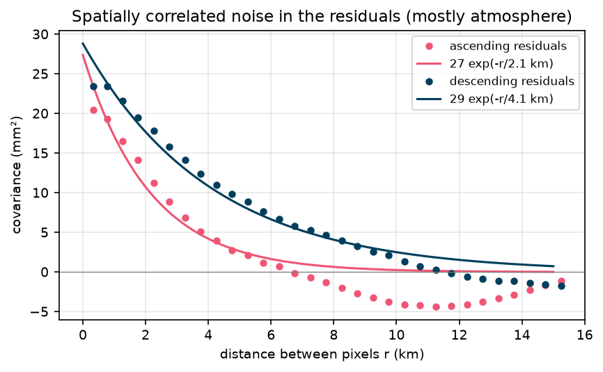

The noise has a standard deviation of about 5 mm and is correlated over 2 km (ascending) to 4 km (descending). A small nugget (10% of σ² on the diagonal) represents uncorrelated pixel noise and keeps the matrix well conditioned. The residuals include any model error as well as noise, so this covariance is, if anything, generous. That is a common and defensible choice.

Step 4: fit the Mogi source and the sill

for kind in ["mogi", "sill"]:
    sol = fit(kind, data, whiten)
    best[kind] = sol.x
    chi2 = 2 * sol.cost
    rms = np.sqrt(np.mean(np.concatenate([(data[k] - predict(kind, sol.x, obs[k], k)) ** 2 for k in obs])))

mogi : x0 (km) -1.19, y0 (km) -1.17, depth (km) 4.28, dV (1e6 m3) 9.33
       centre 63.8716 N, 22.4580 W; volume change 9.33 million m3 in 48 days = 2.25 m3/s; RMS misfit 6.7 mm at the quadtree points; chi2 436 for 1349 points and 10 parameters; 10 evaluations
sill : x0 (km) -1.24, y0 (km) -1.21, depth (km) 4.77, length (km) 5.87, width (km) 0.20, strike (deg) 58.88, opening (m) 6.38
       centre 63.8713 N, 22.4591 W; volume change 7.49 million m3 in 48 days = 1.81 m3/s; RMS misfit 6.0 mm at the quadtree points; chi2 380 for 1349 points and 13 parameters; 118 evaluations

The Mogi source sits 1.7 km south-west of SENG at 4.28 km depth, and grew by 9.33 million m³ in 48 days, 2.25 m³ per second. The sill is centred in almost the same place, 0.5 km deeper, and elongated north-east–south-west over 5.9 km.

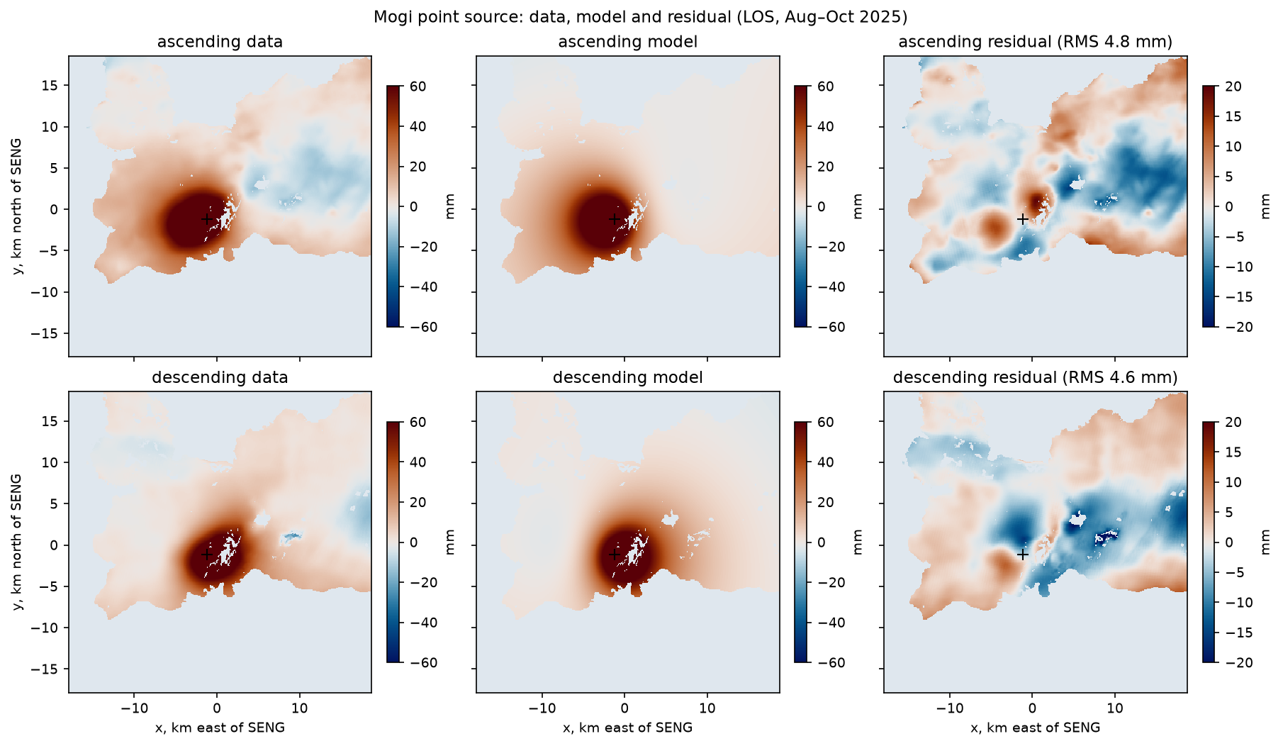
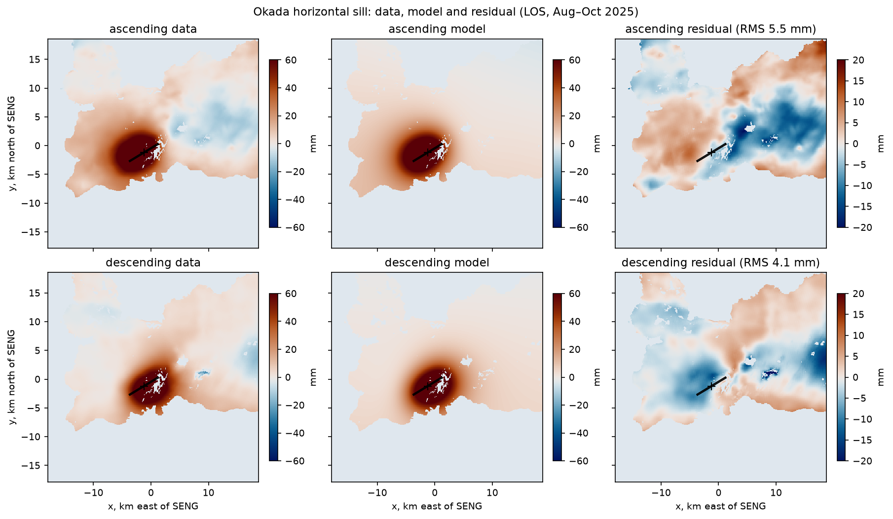
Is the sill really better? It reduces the misfit from 6.7 to 6.0 mm at the quadtree points, and χ² from 436 to 380, for 3 extra parameters. That is a large improvement in χ² terms. But note the width: it went to its lower bound of 0.2 km. The data want a long, narrow source, closer to a horizontal “pipe” than a pancake. A narrow sill and a wide one with less opening produce very similar surface patterns at 4.8 km depth, as the next step shows.

χ² is also much smaller than the number of data (436 against 1,349). This means the covariance overestimates the noise at the quadtree points. That is expected: we estimated it from individual pixels, but each quadtree point is an average of up to several hundred pixels, which reduces the uncorrelated part of the noise. The uncertainties below are therefore on the conservative side.

Step 5: uncertainties by Monte Carlo

The inversion gives one best model. To estimate how much it could change, we draw synthetic noise with exactly the covariance C, add it to the data, and refit, many times. If z is a vector of independent standard normal numbers, then Lz has covariance LLᵀ = C. This is sometimes called a parametric bootstrap.

N_MC = 200                                 # Monte Carlo realisations of correlated noise
RNG = np.random.default_rng(42)

for kind in ["mogi", "sill"]:
    n_mc = N_MC if kind == "mogi" else N_MC // 2
    draws = []
    for _ in range(n_mc):
        noisy = {k: data[k] + chol[k] @ RNG.standard_normal(len(data[k])) for k in obs}
        draws.append(fit(kind, noisy, whiten, p0=best[kind]).x)
    draws = np.array(draws)

mogi  x0 (km)          -1.19  95% interval    -1.37 ..    -1.00  (std 0.10)
mogi  y0 (km)          -1.17  95% interval    -1.31 ..    -1.00  (std 0.08)
mogi  depth (km)        4.28  95% interval     4.04 ..     4.51  (std 0.12)
mogi  dV (1e6 m3)       9.33  95% interval     8.39 ..    10.55  (std 0.61)
mogi  volume (1e6 m3)     9.33  95% interval     8.39 ..    10.55  -> 2.02-2.54 m3/s
sill  x0 (km)          -1.24  95% interval    -1.43 ..    -1.07  (std 0.09)
sill  y0 (km)          -1.21  95% interval    -1.37 ..    -1.07  (std 0.08)
sill  depth (km)        4.77  95% interval     4.29 ..     5.09  (std 0.20)
sill  length (km)       5.87  95% interval     5.18 ..     6.43  (std 0.33)
sill  width (km)        0.20  95% interval     0.20 ..     2.83  (std 0.78)
sill  strike (deg)     58.88  95% interval    51.70 ..    65.87  (std 3.72)
sill  opening (m)       6.38  95% interval     0.40 ..     7.84  (std 2.28)
sill  volume (1e6 m3)     7.49  95% interval     6.85 ..     8.37  -> 1.65-2.02 m3/s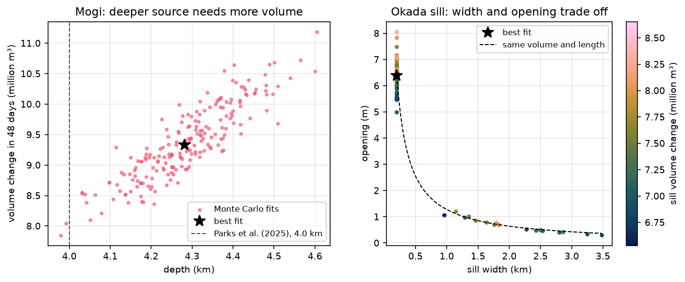

Two lessons stand out, and both are general:

1. Depth and volume are correlated. The Mogi points form a tight band: every 0.1 km of extra depth needs about 0.4–0.5 million m³ more volume, as expected from u_max ∝ ΔV/d². Quoting the two uncertainties separately hides this. Always look at the joint distribution.
2. Some parameters are not resolved. The sill width ranges from 0.2 to 2.8 km and the opening from 0.4 to 7.8 m, but their product, the volume per unit length, is well determined. At 4–5 km depth, InSAR cannot tell a narrow, thick sill from a wide, thin one. The volume, 6.85–8.37 million m³, is robust.

Step 6: compare with published results

mogi : our centre is 0.35 km from the published Mogi location (63.869 N, 22.454 W); depth 4.28 km vs 4.0 km (Mogi) and 4.35-4.7 km (sill)
sill : our centre is 0.35 km from the published Mogi location (63.869 N, 22.454 W); depth 4.77 km vs 4.0 km (Mogi) and 4.35-4.7 km (sill)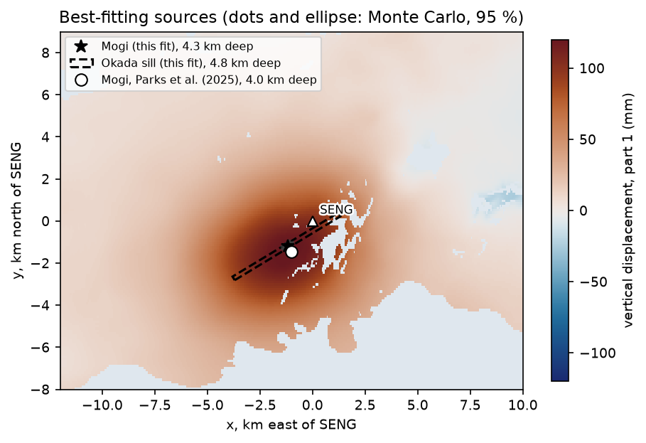

Parks et al. (2025), in Earth and Planetary Science Letters, modelled GNSS and InSAR deformation at Svartsengi associated with the Sundhnúkur crater row eruptions. They found a Mogi source at 63.869° N, 22.454° W and 4.0 km depth, and a sill at 4.35–4.7 km depth. Our fit uses different data (August–September 2025, after the ninth eruption), yet:

• the horizontal position agrees to 0.35 km, which is three to four Monte Carlo standard deviations, a reasonable agreement for a different time window, different data and our simple noise model;
• the Mogi depth of 4.28 km is slightly deeper than their 4.0 km, and the sill depth of 4.77 km is slightly deeper than their 4.35–4.7 km. In both cases, the sill is deeper than the point source, as in their study;
• the inflow rate, 1.8–2.3 m³ per second depending on the model, is at the low end of the 2.4–9 m³/s range they report for the earlier inflation periods. That is consistent with the slower uplift since 2025 seen in the SENG GNSS record in Part 1. The Icelandic Meteorological Office (IMO) estimated about 27.5 million m³ accumulated from mid-July 2025 to early June 2026, an average of about 1 m³ per second, which is lower again because the inflation rate decreases through each cycle.

Limitations and caveats

• Elastic, homogeneous half-space. Real crust is layered, faulted, hot and partly viscoelastic, especially around a long-lived magma reservoir. Layering and heterogeneity can shift the inferred depth and volume. Topography is modest here (a few hundred metres at most) and is ignored.
• One window, two models. We fitted 48 days. A different window might give a slightly different source, and the inflation rate decays through each cycle. Part 3 shows that change.
• Simple noise model. An isotropic exponential covariance, estimated from residuals that include model error, is a standard simplification. Topography-correlated tropospheric delay and anisotropic turbulence are not modelled.
• Local minima. least_squares is a local method. The Mogi fit converged in 10 evaluations from a simple start, but the sill took 118, and more complex models (several sources, dykes) can have multiple minima. Try several starting points, or use a global method such as Bayesian MCMC sampling, for example GBIS (Bagnardi and Hooper, 2018).
• Prior choice. The 0.2 km lower bound on sill width is our choice. The best fit sits on it, so the “best” sill width is really “narrow, unresolved”.
• The far field. Our reference area may contain real deformation from the wider plate boundary. The nuisance ramps absorb some of it, but they can also absorb part of the long-wavelength deformation from a deep source.

Try it yourself

1. Fix the sill width. Set the lower and upper bounds for width to 3 km in START["sill"]. How do the opening, depth and misfit change? Does the volume stay the same?
2. Change the quadtree threshold. Run with quadtree(d, max_std=1.0) and max_std=5.0. How many points do you get, and do the depth and volume change by more than their uncertainties?
3. Ignore the correlated noise. Use eye instead of whiten in the final fit and in the Monte Carlo (and draw uncorrelated noise). How much smaller are the uncertainties? Which result would you publish?
4. Poisson’s ratio. Rerun with NU = 0.30. Which parameters change, and why does the depth not?
5. Model the 1 April 2025 dyke. Use Part 1’s cached and deramp functions to build an ascending LOS map across the eruption from the pair 20250330_20250405, and fit an Okada source with dip fixed at 90° (a vertical dyke) plus a Mogi deflation source. Compare the dyke strike with the line of the Sundhnúkur craters.
6. Joint inversion with GNSS. Add SENG’s 3D displacement from Part 1 as three more observations with 1–4 mm uncertainties. Does it tighten the depth–volume trade-off?

Frequently asked questions

What is the Mogi model?

The Mogi model describes the surface displacement caused by a small spherical source of pressure (or volume change) buried in a uniform elastic half-space. It was popularised by Kiyoo Mogi in 1958 for Japanese volcanoes. It has only four parameters (horizontal position, depth and volume change), gives radially symmetric uplift and outward horizontal motion, and is the most widely used first model for volcanic deformation.

How do you estimate magma chamber depth from InSAR?

Fit a source model to the InSAR displacement. The width of the deformation pattern, not its amplitude, determines the depth: for a Mogi source, uplift falls to half its peak at about 0.77 times the depth. In practice, you downsample the data, project the model into the line of sight, and minimise the misfit with non-linear least squares or Bayesian sampling, accounting for correlated atmospheric noise.

What is the difference between the Mogi and Okada models?

The Mogi model is a point source of volume change, which produces a symmetric bulge. The Okada model is a finite rectangular dislocation that can slip or open, so it can represent faults, dykes and sills with a length, width, strike and dip. For the same volume change, a shallow-dipping sill produces a narrower uplift and twice the peak uplift of a Mogi source, so the choice of model affects the inferred volume and depth.

Why do InSAR inversions use quadtree downsampling?

A single interferogram has hundreds of thousands of pixels, but neighbouring pixels are highly redundant and their noise is correlated. Quadtree downsampling keeps many points where the displacement changes rapidly and few where it is smooth, reducing the data to a few hundred or thousand points. That makes forward modelling fast and the data covariance matrix small enough to invert.

How do you estimate uncertainties for a volcanic source model?

Estimate the data covariance, usually from the residuals or from a non-deforming area, as a function of distance. Then either sample the posterior distribution with a Bayesian method such as Markov chain Monte Carlo, or add many realisations of noise drawn from that covariance to the data and refit each time. The spread of the results gives uncertainties and reveals trade-offs such as depth against volume.

Is the Mogi model realistic?

It is a useful approximation, not a realistic description. Real magma reservoirs have finite size and shape, the crust is layered and not perfectly elastic, and topography matters on steep volcanoes. Even so, a Mogi source often locates the centre of pressure and estimates the volume change well enough for monitoring, and more complex models are judged by how much better they fit.

Next steps

• Part 3: InSAR time series validated with GNSS. Follow the uplift through six inflation phases from 2024 to 2026 and see how the rate has decreased.
• Part 1: mapping volcano deformation with InSAR explains how the LOS maps used here were made.
• Fit a statistical model to spatial data in a different field with kriging spatial interpolation in Python; the covariance fitting in Step 3 is the same idea as a variogram.
• See a non-volcanic InSAR signal in InSAR ground subsidence in Python.

Data and licences

• COMET LiCSAR products: contain modified Copernicus Sentinel data 2025, processed by COMET (LiCSAR). Open data under CC BY 4.0. Frames 016A_02504_162118 and 155D_02484_191814.
• References: Mogi, K. (1958), “Relations between the eruptions of various volcanoes and the deformations of the ground surfaces around them”, Bulletin of the Earthquake Research Institute 36, 99–134; Okada, Y. (1985), “Surface deformation due to shear and tensile faults in a half-space”, Bulletin of the Seismological Society of America 75(4), 1135–1154; Parks, M. et al. (2025), Earth and Planetary Science Letters 658, 119324, doi:10.1016/j.epsl.2025.119324; Bagnardi, M. and Hooper, A. (2018), “Inversion of surface deformation data for rapid estimates of source parameters and uncertainties: a Bayesian approach”, Geochemistry, Geophysics, Geosystems 19, 2194–2211; Rivalta, E. and Segall, P. (2008), “Magma compressibility and the missing source for some dike intrusions”, Geophysical Research Letters 35, L04306; Lazecký, M. et al. (2020), Remote Sensing 12(15), 2430; Icelandic Meteorological Office news updates (vedur.is), 2025–2026.
• Code: mogi_okada_inversion.py, tested with Python 3.12.0, NumPy 2.5.4, SciPy 1.18.1, rasterio 1.5.2, Matplotlib 3.11.2 and cmcrameri 1.10.