Kriging in Python with PyKrige: IDW vs ordinary kriging of UK NO₂ monitoring data
A practical spatial interpolation tutorial in Python: download real 2025 NO₂ annual means from the UK AURN network, fit spherical, exponential and Gaussian variograms, run ordinary kriging with PyKrige, compare it with inverse distance weighting, score both with leave-one-out cross-validation, map the kriging variance and add Sentinel-5P satellite NO₂ as a covariate.
- Level
- Intermediate
- Tested with
- Python 3.12
- Source code
- Download scripts
Key takeaways
- Ordinary kriging fits a variogram to the data and uses it to weight neighbours; IDW uses a fixed distance rule. Both are a few lines with NumPy and PyKrige.
- On 74 UK background NO₂ stations from 2025, the spherical variogram had a nugget of 18.8 and a sill of 30.5 (µg/m³)²: 62% of the variance is local and does not depend on distance.
- Leave-one-out cross-validation gave the same RMSE for IDW (power 2) and ordinary kriging, 4.80 µg/m³, against 5.26 for simply using the mean. Kriging had almost no bias (+0.07) where IDW over-predicted by 0.98.
- The kriging standard deviation was 4.6–5.7 µg/m³ and well calibrated: 95% of left-out stations fell inside the 95% interval.
- Adding the Sentinel-5P NO₂ column from Part 1 as a covariate cut the RMSE to 3.53 µg/m³. Column and surface agree well at background sites (r = 0.75) but poorly at roadside sites (r = 0.40).
Before you start
- Comfortable with NumPy, pandas and GeoPandas (see Getting started with GeoPandas)
- Python 3.10+ with PyKrige, pyreadr, numpy, scipy, pandas, geopandas, rasterio, requests and matplotlib
- Optional for Step 7: the Sentinel-5P annual NO₂ GeoTIFF from Part 1 of this series, made by one command
Short answer: to krige in Python, put your points in a projected coordinate system and create OrdinaryKriging(x, y, z, variogram_model="spherical") from PyKrige. It computes the experimental variogram and fits the model for you. Then call .execute("grid", gx, gy), which returns the predictions and the kriging variance for every cell. For IDW, a weighted mean with weights 1/dᵖ takes five lines of NumPy. Choose between them with leave-one-out cross-validation: predict each point from all the others and compare the RMSE. On real UK NO₂ data, the two methods scored the same RMSE (4.80 µg/m³). Kriging was unbiased and gave a calibrated uncertainty map. A satellite covariate did much better than either.
Spatial interpolation turns measurements at a few points, such as weather stations, rain gauges, boreholes or air-quality monitors, into a continuous surface. It is one of the most common tasks in GIS, and one of the easiest to do badly: every method draws a smooth, convincing map, whether or not the data support it. This tutorial uses real NO₂ measurements from the UK’s national monitoring network to show how to choose a method, check it honestly and say how uncertain the map is.
You will learn how to:
- download AURN annual mean NO₂ for 2025 from Defra’s UK-AIR with
pyreadr, and choose which stations to interpolate; - compute an experimental variogram and fit spherical, exponential and Gaussian models;
- run ordinary kriging with PyKrige on a 2 km grid over the UK;
- write IDW in NumPy and compare the two maps;
- run leave-one-out cross-validation and compare RMSE, MAE and bias;
- map the kriging standard deviation and check whether it is calibrated;
- add the Sentinel-5P satellite NO₂ column as a covariate with regression kriging, and see what the column-versus-surface mismatch means.
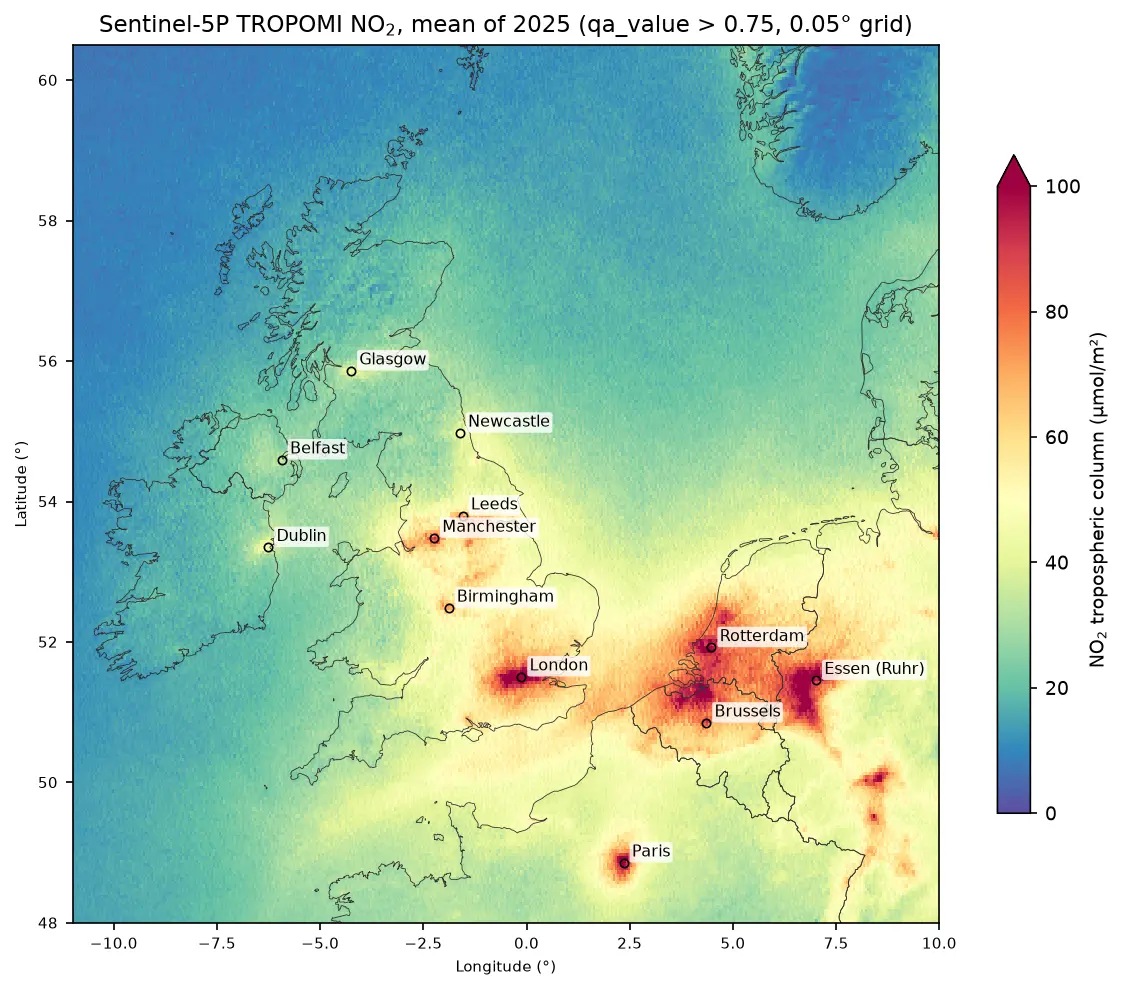
This is Part 2 of a series. Part 1, Sentinel-5P NO₂ in Python, makes the satellite NO₂ map used in Step 7. Steps 1–6 do not need it.
All outputs below are real results from kriging_no2_uk.py, run on 19 October 2026 with Python 3.12, PyKrige 1.7.3, pyreadr 0.5.7, geopandas 1.2.0 and rasterio 1.5.2.
IDW or kriging: what is the difference?
Both methods predict a value at an unsampled location as a weighted average of the observations. They differ in how they choose the weights:
| Inverse distance weighting (IDW) | Ordinary kriging | |
|---|---|---|
| Weights | 1 / distanceᵖ, fixed by you | Solved from a variogram fitted to the data |
| Clustered stations | Each counts fully, so clusters dominate | Down-weighted, because they carry overlapping information |
| Passes through the data | Always | Only if the nugget is zero |
| Uncertainty | None | Kriging variance at every cell |
| Assumptions | None stated | Stationary mean and variogram |
Kriging is “optimal” only if its variogram describes the data well. The rest of this tutorial is about checking that.
Step 1: download the AURN annual means
Defra publishes AURN data for the openair R package as .rds and .RData files on UK-AIR, with no login. pyreadr reads them into pandas. One file has the 2025 annual statistics for every station, the other has the site metadata: coordinates, the environment type (traffic, urban background, rural and so on) and the date to which data are ratified.
YEAR = 2025UKAIR = "https://uk-air.defra.gov.uk/openair/R_data/"
annual = pyreadr.read_r(fetch(f"summary_annual_AURN_{YEAR}.rds"))[None]meta = pyreadr.read_r(fetch("AURN_metadata.RData"))["AURN_metadata"]meta = meta[meta["parameter"] == "NO2"].drop_duplicates("site_id")aurn = (annual[["code", "site", "NO2.mean", "NO2.capture"]] .rename(columns={"NO2.mean": "no2", "NO2.capture": "capture"}) .merge(meta[["site_id", "location_type", "latitude", "longitude", "ratified_to"]], left_on="code", right_on="site_id", how="left") .drop(columns="site_id"))aurn = aurn[aurn["no2"].notna()]158 stations report NO2; 143 have >= 75% data captureratified to: {'2026-06-30': 154, '2026-03-31': 1} count mean min maxlocation_typeRural Background 12 5.0 1.5 10.7Suburban Background 3 9.9 6.5 16.4Suburban Industrial 2 14.1 13.8 14.4Urban Background 59 13.5 4.2 24.8Urban Industrial 6 13.2 9.3 21.7Urban Traffic 60 20.4 8.3 34.8Almost all 2025 data are ratified (quality-checked) to mid-2026, so these are final values. We keep stations with at least 75% data capture, the usual threshold for a valid annual mean.
The most important decision in this tutorial comes next: which stations to interpolate. Traffic stations measure the air a few metres from a busy road. Their values change over tens of metres and depend on the road, not on the region, so interpolating between traffic stations 20 km apart would produce a meaningless surface. We interpolate only background stations, which represent the general air people breathe away from roads, and keep the 60 traffic stations aside as a test.
BACKGROUND = ["Urban Background", "Suburban Background", "Rural Background"]stations = aurn[(aurn["capture"] >= 0.75) & aurn["location_type"].isin(BACKGROUND)].copy()roadside = aurn[(aurn["capture"] >= 0.75) & (aurn["location_type"] == "Urban Traffic")].copy()CRS = "EPSG:27700" # British National Grid, metresgdf = gpd.GeoDataFrame(stations, geometry=gpd.points_from_xy(stations.longitude, stations.latitude), crs="EPSG:4326").to_crs(CRS)x, y, z = gdf.geometry.x.to_numpy() / 1000, gdf.geometry.y.to_numpy() / 1000, gdf["no2"].to_numpy() # kmAlways interpolate in a projected coordinate system with equal units on both axes. Distances in degrees of longitude and latitude are not equal (at 54° N a degree of longitude is only 59% as long as a degree of latitude), which would distort both IDW and the variogram. We use the British National Grid and work in kilometres to keep the numbers readable.
kept 74 background stations: mean 12.0, sd 5.2, range 1.5 to 24.8 ug/m3nearest-neighbour distance: median 17.9 km, max 217.8 km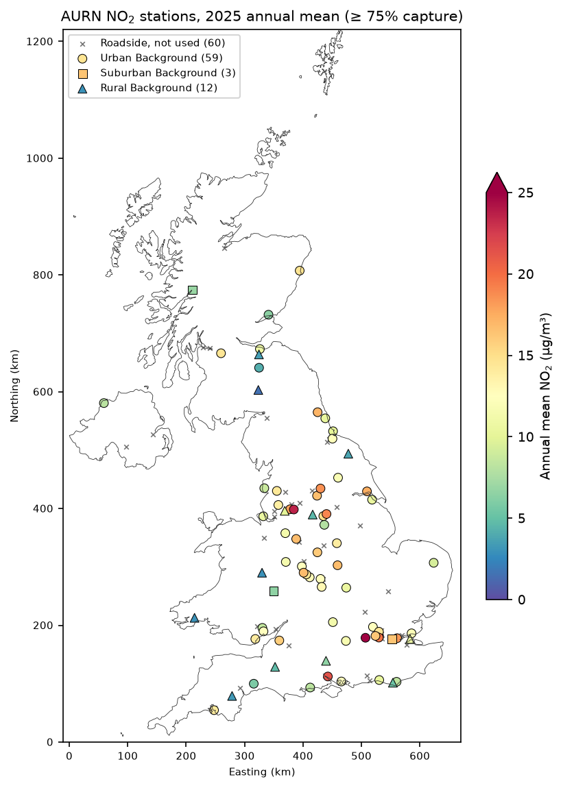
Step 2: fit the variogram
The experimental variogram groups all pairs of stations by their separation distance and computes half the mean squared difference in each distance bin (lag). If nearby stations are more alike than distant ones, it rises with distance and then levels off. PyKrige computes it when you create an OrdinaryKriging object and fits the chosen model by weighted least squares:
NLAGS = 12MODELS = ["spherical", "exponential", "gaussian"]fits = {}for model in MODELS: ok = OrdinaryKriging(x, y, z, variogram_model=model, nlags=NLAGS, weight=True) fits[model] = ok psill, rng, nugget = ok.variogram_model_parametersweight=True gives more weight to the short lags in the fit, which matter most for prediction. PyKrige returns the partial sill, so the total sill is the partial sill plus the nugget.
spherical partial sill 11.69 range 342.9 km nugget 18.84 -> nugget/sill 0.62exponential partial sill 14.65 range 636.1 km nugget 18.55 -> nugget/sill 0.56gaussian partial sill 10.02 range 333.1 km nugget 20.94 -> nugget/sill 0.68lag centres (km): [40, 100, 162, 228, 288, 352, 412, 478, 542, 607, 668, 727]semivariance: [20.9, 25.9, 21.2, 30.8, 31.6, 31.4, 22.7, 36.7, 31.5, 28.2, 27.8, 17.1]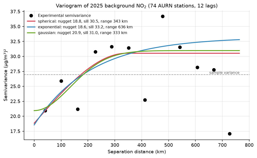
This is a real-world variogram, and it is not the textbook curve. Three things stand out:
- A large nugget. The semivariance at the shortest lag (40 km) is already 20.9, and the models put the nugget at about 19, which is 56–68% of the sill. Most of the variation between background stations is local: an urban background site in a city centre and a suburban one 10 km away differ because of their surroundings, not because of their distance.
- A noisy curve. The 74 stations make 2,701 pairs, about 225 per lag and mostly from the dense cluster in England, so the points jump around. The last lags (above about 600 km) compare southern England with northern Scotland and should be given little attention.
- Similar fits. The three models are almost the same where the data are. The spherical model is a sensible default; we test whether the choice matters in Step 5.
Step 3: ordinary kriging on a 2 km grid
We predict on a 2 km grid in British National Grid coordinates that covers the whole UK, and mask it to land with the Natural Earth outline:
CELL = 2000X0, Y1 = 0, 1_220_000GX, GY = 330, 610                                         # 660 km x 1220 km at 2 kmgx = (X0 + CELL * (np.arange(GX) + 0.5)) / 1000gy = (Y1 - CELL * (np.arange(GY) + 0.5)) / 1000transform = from_origin(X0, Y1, CELL, CELL)on_land = ~geometry_mask(uk.geometry, (GY, GX), transform)
MODEL = "spherical"ok = fits[MODEL]z_ok, var_ok = ok.execute("grid", gx, gy, backend="vectorized")z_ok, var_ok = np.asarray(z_ok), np.asarray(var_ok)sd_ok = np.sqrt(np.clip(var_ok, 0, None))
execute("grid", ...) returns two arrays: the predictions and the kriging variance. The vectorized backend solves every cell in one matrix operation, which is fast for a few hundred stations; for thousands of points use backend="loop" with n_closest_points to limit each prediction to its nearest neighbours.
330 x 610 cells of 2 km, 60,917 on landspherical model, 0.5 s for 201,300 cellsland cells: predicted NO2 6.9 to 15.8 ug/m3; kriging SD 4.6 to 5.7 (median 4.9)The data range from 1.5 to 24.8 µg/m³, but the kriged surface ranges only from 6.9 to 15.8. That is the large nugget at work: kriging treats most of each station’s difference from its neighbours as local noise and pulls predictions towards the regional mean.
Step 4: IDW, and the two maps side by side
Inverse distance weighting needs no library. Each cell gets a weighted mean of all stations, with weights 1/dᵖ:
def idw(xs, ys, zs, xq, yq, power=2.0):    """Inverse distance weighting: a weighted mean of every station, with weights 1 / d^power."""    d = np.hypot(xq[:, None] - xs[None, :], yq[:, None] - ys[None, :])    d = np.maximum(d, 1e-6)    w = 1.0 / d ** power    return (w @ zs) / w.sum(1)

GXX, GYY = np.meshgrid(gx, gy)z_idw = idw(x, y, z, GXX.ravel(), GYY.ravel(), 2).reshape(GY, GX)land cells: 1.5 to 24.8 ug/m3kriging minus IDW over land: mean -0.51, 5th to 95th percentile -2.6 to +1.8 ug/m3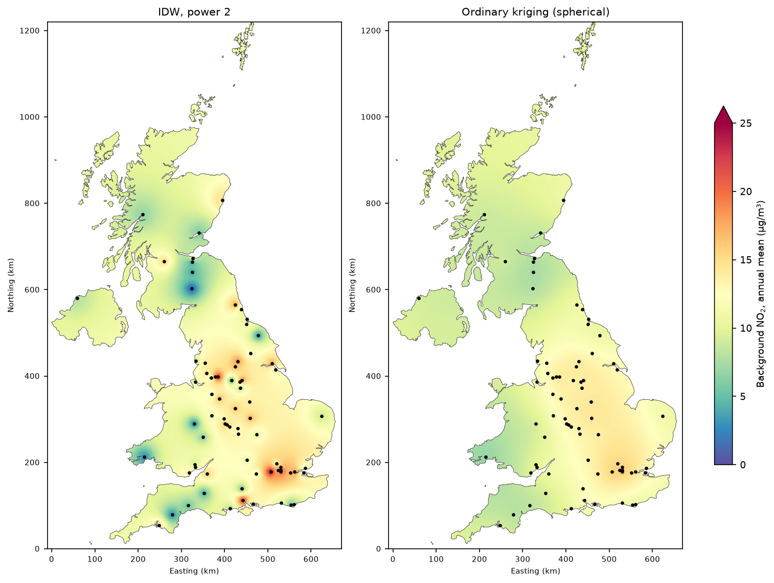
The maps look very different. IDW always passes exactly through every observation, so a single rural station with 3 µg/m³ in the Lake District or Wales becomes a blue bullseye, and a city-centre background site becomes a red spot. Far from any station, IDW drifts towards the mean of all stations, which is dominated by the dense, polluted English cluster. Kriging produces a smooth regional surface: higher over London and the Midlands, lower over Scotland, Wales and Northern Ireland. Which is better? A map cannot tell you. Cross-validation can.
Step 5: leave-one-out cross-validation
Leave-one-out cross-validation (LOOCV) removes each station in turn, predicts it from the other 73, and compares the prediction with the measurement. We score IDW with powers 1, 2 and 3, kriging with each variogram model, and the simplest possible baseline, the mean of the other stations:
def loo(predict):    pred = np.empty(n)    for i in range(n):        keep = np.arange(n) != i        pred[i] = predict(keep, i)    return pred

def ok_loo(model):    psill, rng, nugget = fits[model].variogram_model_parameters   # variogram fixed from the full data set    params = {"psill": psill, "range": rng, "nugget": nugget}
    def predict(keep, i):        m = OrdinaryKriging(x[keep], y[keep], z[keep], variogram_model=model,                            variogram_parameters=params)        p, v = m.execute("points", x[i:i + 1], y[i:i + 1])        ok_var[model][i] = v[0]        return p[0]    return predict

ok_var = {m: np.empty(n) for m in MODELS}preds = {"Global mean": loo(lambda k, i: z[k].mean())}for p in (1, 2, 3): preds[f"IDW p={p}"] = loo(lambda k, i, p=p: idw(x[k], y[k], z[k], x[i:i + 1], y[i:i + 1], p)[0])for m in MODELS: preds[f"OK {m}"] = loo(ok_loo(m)) RMSE MAE bias rIDW p=2 4.80 4.03 0.98 0.45OK spherical 4.80 3.93 0.07 0.38OK exponential 4.80 3.91 0.07 0.38IDW p=1 4.82 3.94 0.68 0.43OK gaussian 4.93 4.04 0.04 0.32IDW p=3 5.05 4.29 1.05 0.44Global mean 5.26 4.18 -0.00 NaNOK spherical: mean standardised error +0.01, SD of standardised error 1.00 (1.0 = kriging variance is well calibrated)share of stations inside the 95% kriging interval: 95%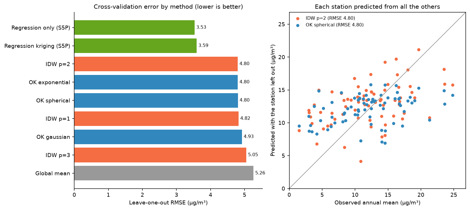
The honest result: IDW with power 2 and ordinary kriging have the same RMSE, 4.80 µg/m³, and both are only about 9% better than predicting every station with the national mean (5.26). That is what the variogram told us to expect. With a nugget that is 62% of the sill, neighbours carry little information about each other, so no interpolator can do much better.
The details still favour kriging:
- Bias. IDW over-predicts by 0.98 µg/m³ on average, because the many stations in polluted English cities dominate its weights everywhere. Kriging’s declustering removes this (+0.07).
- MAE. Kriging’s typical error is slightly smaller (3.91–3.93 against 4.03).
- Calibrated uncertainty. The standardised errors have a mean of +0.01 and a standard deviation of 1.00, and exactly 95% of left-out stations fall inside their 95% kriging interval. The kriging variance is telling the truth, which IDW cannot do at all.
- IDW power matters. Power 3 (5.05) is worse than power 1 or 2, because it trusts the nearest station too much when the nearest station is mostly local noise.
We kept the variogram fitted to all 74 stations for every fold. Strictly, a fully independent test would refit it without the left-out station; with 74 stations the difference is small, but the scores are very slightly optimistic for kriging.
The largest errors show where the method breaks down:
site type observed OK IDW p=2 OK error Southampton Centre Urban Background 21.3 10.4 10.8 -10.9Manchester Piccadilly Urban Background 23.6 12.9 15.9 -10.7 London Hillingdon Urban Background 24.8 14.2 15.8 -10.6 Ladybower Rural Background 4.5 14.8 15.0 10.3 High Muffles Rural Background 3.8 12.5 12.7 8.7 London Bloomsbury Urban Background 23.5 14.9 18.1 -8.6They are city-centre sites under-predicted by about 10 µg/m³ (London Hillingdon is close to Heathrow and the M4), and rural sites in the Peak District and the North York Moors over-predicted by similar amounts. In both cases the station’s surroundings, not its position, set its value. And for the roadside stations we left out:
60 roadside stations: observed mean 20.4, background kriging at the same points 12.1 ug/m3 (under-prediction 8.3)The background surface under-predicts roadside NO₂ by 8.3 µg/m³ on average. That is expected and correct: the map shows background air, and the roadside increment has to come from a traffic model or local measurements.
Step 6: map where the kriging is least certain
sd_ok = np.sqrt(np.clip(var_ok, 0, None))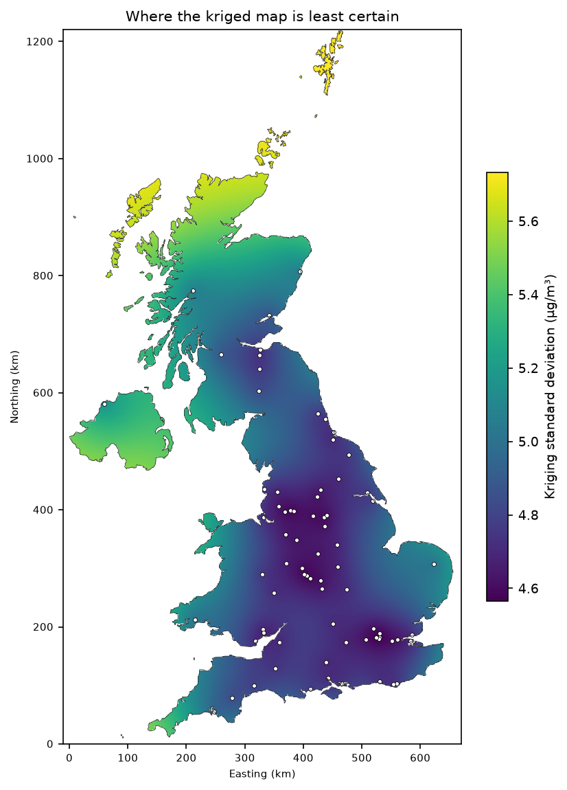
The kriging standard deviation ranges from 4.6 µg/m³ in the station clusters to 5.7 in Shetland. The range is narrow because of the large nugget: even right next to a station, kriging cannot know the local part of the variation, so the uncertainty never falls close to zero. Note that the kriging variance depends only on where the stations are and on the variogram, not on the values measured. It shows where you need more stations, but it will not warn you that the surface is wrong near an unusual source, such as an airport.
Step 7: add the Sentinel-5P column as a covariate
Kriging struggles because most of the variation is local. A satellite NO₂ map, which sees every location, can supply that local information. The script samples the 2025 Sentinel-5P annual mean from Part 1 at every station and at every grid cell, fits a linear regression of surface NO₂ on the column, and kriges the residuals. This is regression kriging. We also test the regression on its own.
S5P = HERE.parent / "sentinel-5p-no2-air-pollution-python" / "output" / f"s5p_no2_{YEAR}_mean.tif"with rasterio.open(S5P) as src:    lonlat = gdf.to_crs("EPSG:4326").geometry    col = np.array([v[0] for v in src.sample(zip(lonlat.x, lonlat.y), indexes=1)])
def rk_predict(keep, i):    b1, b0 = np.polyfit(col[keep], z[keep], 1)    res = z[keep] - (b0 + b1 * col[keep])    m = OrdinaryKriging(x[keep], y[keep], res, variogram_model="spherical", nlags=NLAGS, weight=True)    return b0 + b1 * col[i] + m.execute("points", x[i:i + 1], y[i:i + 1])[0][0]
preds["Regression kriging (S5P)"] = loo(rk_predict)preds["Regression only (S5P)"] = loo(lambda k, i: np.polyval(np.polyfit(col[k], z[k], 1), col[i]))
The regression and the residual variogram are refitted inside every fold, so this test is fully independent.
background stations: Pearson r = 0.75, NO2 = 2.09 + 0.169 x column (umol/m2)roadside stations:   Pearson r = 0.40
LOOCV including the satellite covariate:                          RMSE   MAE  bias     rRegression only (S5P)     3.53  2.82  0.01  0.73Regression kriging (S5P)  3.59  2.80  0.00  0.72OK spherical              4.80  3.93  0.07  0.38IDW p=2                   4.80  4.03  0.98  0.45residual variogram: partial sill 3.64, range 465.9 km, nugget 9.37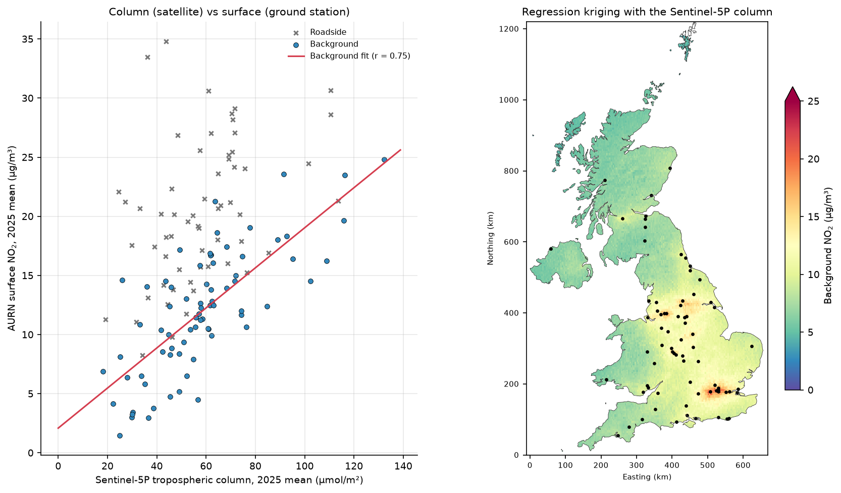
The satellite column is a much better predictor than distance. The regression alone cuts the RMSE from 4.80 to 3.53 µg/m³, 26% better than kriging. Kriging the residuals adds nothing (3.59): after the satellite explains the regional and urban pattern, the residual variogram is almost flat (nugget 9.37 against a partial sill of 3.64), so the leftover errors are local to each site.
Be honest about the column–surface mismatch
A correlation of 0.75 is good, but the two quantities are not the same thing, and the comparison has several mismatches that you should state whenever you combine them:
- Column versus concentration. Sentinel-5P measures molecules in the whole tropospheric column (µmol/m²); AURN measures the concentration at about 2 m above the ground (µg/m³). The regression slope, 0.169 µg/m³ per µmol/m², is the same as spreading the column evenly through a layer only about 270 m deep (46 g/mol ÷ 0.169). That is a statistical summary of profile shape, mixing depth and satellite bias, not a physical boundary-layer height.
- Scale. One 0.05° grid cell is about 18 km², while a monitor samples the air within tens to hundreds of metres. That is why roadside sites (r = 0.40) sit far above the line: their extra NO₂ comes from one road, invisible at the satellite’s scale.
- Time. The satellite sees about 13:30 local time on clear days only; AURN measures every hour of every day. Rush hours, nights and cloudy, often windy, days are missing from one side of the comparison.
- Satellite bias. TROPOMI columns are biased low over polluted cities, as Part 1 explains. A regression absorbs a constant bias, but not one that varies with pollution level.
So the regression map is a better estimate of annual mean background NO₂ than either interpolator, but it is still not a compliance map, and it cannot predict roadside concentrations.
Pitfalls and limitations
- Few points. A variogram from 74 stations is noisy, and the long-distance lags rest on a handful of pairs. As a rule of thumb, kriging needs at least 50–100 points; with fewer, IDW or a regression model is often as good.
- Stationarity. Ordinary kriging assumes the same mean and variogram everywhere. Urban and rural NO₂ behave differently, which is one reason the nugget is so large. Covariates (Step 7), or separate models for urban and rural stations, address this.
- Mixing station types. Interpolating traffic and background stations together is the most common error in air-quality interpolation. Decide what your surface represents before choosing stations.
- Projected coordinates. Never krige in degrees of latitude and longitude over large areas. Use a projected CRS, or PyKrige’s
coordinates_type="geographic"for global data. - Variogram fitting. PyKrige’s automatic fit is convenient but not always sensible. Plot the experimental variogram every time, and fix parameters by hand if the fit is driven by a few noisy long lags.
- LOOCV optimism. We used one variogram for all kriging folds. Refitting it inside each fold, as we did for regression kriging, is stricter. For clustered networks, spatial block cross-validation is stricter still.
- One year. Annual means from 2025 only. A different year, or monthly means, would give a different variogram.
Frequently asked questions
Is kriging better than IDW?
Not automatically. Kriging is the best linear unbiased predictor only when its variogram is right, and its advantages are greatest when the data have strong spatial structure and a small nugget. On our UK NO₂ stations, with a nugget of 62% of the sill, ordinary kriging and IDW had the same leave-one-out RMSE (4.80 µg/m³). Kriging was unbiased and gave a calibrated uncertainty map, which IDW cannot do. Always compare methods with cross-validation on your own data.
What is a variogram in kriging?
A variogram (or semivariogram) plots half the mean squared difference between pairs of observations against the distance between them. It usually rises with distance and levels off at the sill; the distance where it levels off is the range, and the value at almost zero distance is the nugget. Kriging uses a model fitted to the variogram to decide how much weight each neighbour gets.
How do I choose the IDW power?
Test several powers with cross-validation and pick the one with the lowest error. Power 2 is the usual default. Higher powers make the surface follow the nearest station more closely, which helps when nearby points are strongly related and hurts when they are noisy. In this tutorial, power 2 (RMSE 4.80) beat power 1 (4.82) narrowly and power 3 (5.05) clearly.
What is the difference between ordinary kriging and universal kriging?
Ordinary kriging assumes an unknown but constant mean across the area. Universal kriging, or kriging with external drift, models the mean as a function of coordinates or of covariates such as elevation or satellite data, and kriges the residuals. Regression kriging, used in Step 7, is a closely related two-step version. PyKrige provides UniversalKriging and, for covariates, RegressionKriging with scikit-learn models.
What does the kriging variance tell me?
It is the expected squared prediction error at each location, given the variogram and the station layout. Its square root, the kriging standard deviation, can be used to draw prediction intervals. It depends on where the stations are, not on the values measured, so it tells you where more stations would help most. Check that it is calibrated with cross-validation: here 95% of left-out stations fell within their 95% interval.
Can I use satellite NO₂ to estimate ground-level NO₂?
Yes, as a covariate, but not by direct conversion. A satellite column is the number of NO₂ molecules from the ground to the top of the troposphere, not the concentration near the ground. Combined with ground stations in a regression, the 2025 Sentinel-5P annual mean explained 56% of the variance in UK background NO₂ and cut the cross-validation RMSE by 26% compared with kriging. It does not capture roadside concentrations.
Next steps
- Make the satellite map yourself in Part 1: Sentinel-5P NO₂ in Python, and try other years or seasons.
- Add more covariates, such as population density, road length within 1 km and elevation, in a land-use regression model; build the road layer with street networks with OSMnx.
- Krige terrain-related data, such as rainfall or temperature, with elevation as external drift; the DEM handling is in Raster terrain analysis with rasterio.
- Revise points, projections and joins in Getting started with GeoPandas, and publish the surfaces on an interactive map with Folium.
Data and licences
- AURN annual statistics and site metadata, 2025: © Crown copyright, Defra, via UK-AIR, licensed under the Open Government Licence v3.0. Files
summary_annual_AURN_2025.rdsandAURN_metadata.RData, accessed on 19 October 2026; data ratified to 30 June 2026. - Sentinel-5P TROPOMI NO₂ (Step 7): contains modified Copernicus Sentinel data 2025, processed by ESA and KNMI, via the Microsoft Planetary Computer and AWS Open Data; see Part 1.
- UK outline: Natural Earth, public domain.
- Software: Murphy, B., Yurchak, R. and Müller, S., PyKrige, BSD licence.
- Code:
kriging_no2_uk.py, tested with Python 3.12.0, PyKrige 1.7.3, pyreadr 0.5.7, numpy 2.5.4, scipy 1.18.1, pandas 3.0.6, geopandas 1.2.0 and rasterio 1.5.2.
Key terms
- Kriging
- A family of geostatistical interpolation methods that predict a value at an unsampled location as a weighted average of nearby observations, with weights chosen from a variogram model to give the best linear unbiased prediction and its variance.
- Variogram (semivariogram)
- A function that describes how different two observations are expected to be, as half the mean squared difference, depending on the distance between them.
- Nugget, sill and range
- The nugget is the semivariance at almost zero distance (measurement error and very local variation); the sill is the level at which the variogram flattens; the range is the distance at which it reaches the sill, beyond which observations are uncorrelated.
- IDW
- Inverse distance weighting: a deterministic interpolator that predicts a weighted mean of observations, with weights proportional to 1 / distance^p.
- LOOCV
- Leave-one-out cross-validation: predict each observation from all the others and compare, giving an honest error estimate for interpolators that would otherwise reproduce the data exactly.
- AURN
- The Automatic Urban and Rural Network, the UK's main network of continuous air-quality monitoring stations, run for Defra and the devolved administrations.
Data for this tutorial
- Defra UK-AIR · AURN annual mean NO₂ for every station (Open Government Licence v3.0)
- Natural Earth · UK outline for the prediction grid
- Microsoft Planetary Computer · Sentinel-5P NO₂ used in Step 7 (via Part 1)
Licences and formats for each source are listed in the GIS data sources catalogue.