Geographically weighted regression in Python: GWR and MGWR with mgwr
Fit geographically weighted regression (GWR) and multiscale GWR (MGWR) in Python with the mgwr package on real West Yorkshire house prices: choose the bandwidth by AICc, map local coefficients with a multiple-testing correction, read local R² and local collinearity, and compare against global OLS, spatial lag and spatial error models.
- Level
- Advanced
- Tested with
- Python 3.12
- Source code
- Download scripts
Key takeaways
- GWR fits a separate weighted regression at every location, so each coefficient becomes a map. In Python, `Sel_BW(coords, y, X).search()` chooses the bandwidth by AICc and `GWR(coords, y, X, bw).fit()` fits the model.
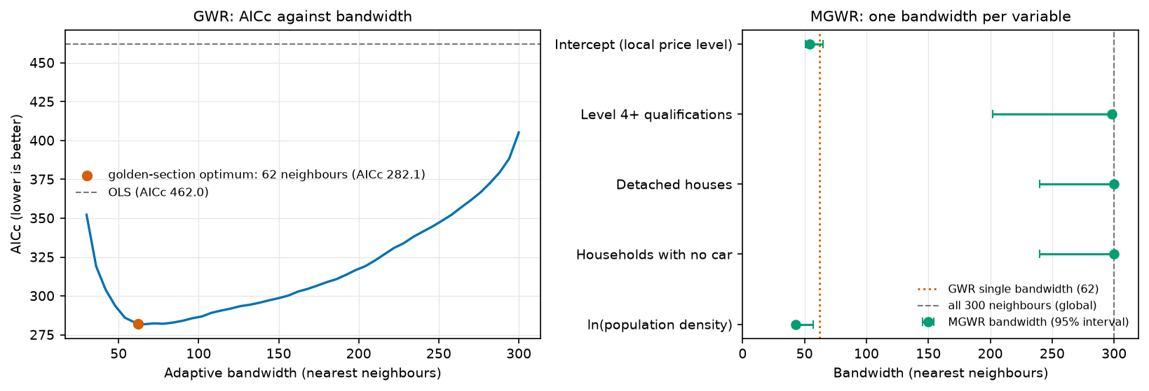
- For median house prices in West Yorkshire's 301 MSOAs, the AICc-optimal GWR uses the 62 nearest neighbours. It raises R² from 0.74 (OLS) to 0.91 and cuts AICc from 462.0 to 282.1, better than the spatial error model's 301.7.
- Local t-tests need a multiple-testing correction. With 56.5 effective parameters, mgwr's corrected critical |t| is 2.87, not 1.97. Applying it cuts the MSOAs where 'detached houses' is significant from 42 to 1.
- MGWR gives each variable its own bandwidth, and here that changes the story. Only the intercept (54 neighbours) and population density (43) vary locally; qualifications, detached houses and car ownership get bandwidths of 298–300 of 300, so their effects are effectively global. MGWR has the best AICc of all (250.0).
- GWR is exploratory. Local coefficients are correlated with each other and with the bandwidth, local collinearity can inflate them (the largest local VIF here is 13.0), and the MGWR bandwidth search took 111 s against 5 s for GWR on only 301 areas.
Before you start
- Comfortable with ordinary least squares regression and with GeoPandas
- Part 1 of this series is helpful but not required: the shared wy_data.py script rebuilds its dataset with one command
- Python 3.10+ with geopandas, pyogrio, libpysal, esda, spreg, mgwr, numpy, pandas, matplotlib, requests and openpyxl
- An internet connection on the first run (about 60 MB of ONS, Nomis and ONS Open Geography downloads) and about two minutes of computing time for MGWR
Short answer: to run geographically weighted regression in Python, install mgwr (part of PySAL). Choose the bandwidth with Sel_BW(coords, y, X).search(criterion="AICc"), fit with GWR(coords, y, X, bw).fit(), and map the columns of results.params. For MGWR, use Sel_BW(coords, y, X, multi=True) and MGWR(coords, y, X, selector).fit(), which give each variable its own bandwidth. Before mapping significance, call results.filter_tvals() with no arguments: that applies mgwr’s corrected critical t-value for multiple testing. For house prices in West Yorkshire, MGWR finds that only the local price level and the effect of population density vary across the county; the other three effects are effectively global.
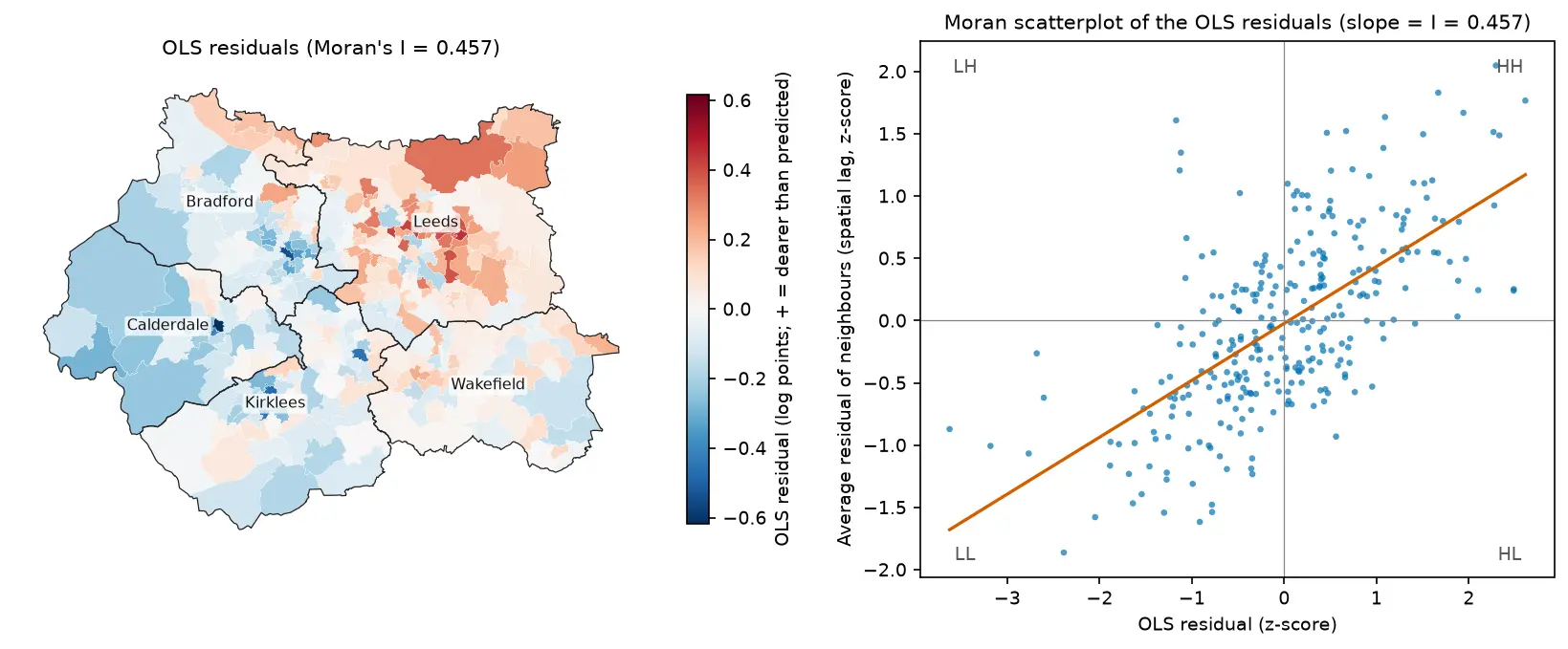
Part 1 of this series fitted global spatial regression models to median house prices in West Yorkshire’s 301 MSOAs. The OLS residuals were strongly clustered (Moran’s I = 0.457), and a spatial error model fitted much better. But all of those models assume that the effect of, say, the share of graduates on prices is the same everywhere: in Ilkley, in inner Bradford and in Wakefield.
Geographically weighted regression drops that assumption. It fits a separate regression around every MSOA, weighting nearby MSOAs more heavily, so each coefficient becomes a surface you can map. This makes it a powerful exploratory tool, and an easy one to over-interpret.
In this tutorial you will:
- prepare the data and coordinates for mgwr, and refit the Part 1 global models on the same scale;
- choose a GWR bandwidth by AICc and see the AICc curve;
- fit GWR and map the local coefficients, greying out MSOAs that are not significant after correcting for multiple testing;
- fit MGWR with one bandwidth per variable and read its bandwidth intervals;
- map the local R² and check local multicollinearity with condition numbers and VIFs;
- compare GWR and MGWR with the OLS, spatial lag and spatial error models from Part 1.
All outputs below are real results from geographically_weighted_regression.py, run in October 2026 with Python 3.12.0, mgwr 2.2.1, spreg 1.9.1, libpysal 4.15.1, esda 2.10.0, geopandas 1.2.0 and numpy 2.5.4.
What you need from Part 1
This part uses exactly the same data as Part 1: the ONS median price paid for all dwellings in the year ending March 2026 for each 2021 MSOA (the successor to HPSSA dataset 2), and four Census 2021 variables from Nomis:
level4: % of residents aged 16+ with a Level 4+ (degree-level) qualification;detached: % of households in a detached house;no_car: % of households with no car or van;ln_density: the log of residents per km².
You do not need to have run Part 1. The code folder contains the same wy_data.py module, which downloads the price workbook, the four Nomis bulk tables and the ONS MSOA 2021 boundaries, joins them, and caches data/west_yorkshire_msoa.gpkg. Run it once:
pip install -r requirements.txtpython wy_data.py301 MSOAs in West Yorkshire; 0 without a median price; written to data\west_yorkshire_msoa.gpkgThe GWR script imports load_west_yorkshire() from the same module, so it also builds the file on first use if you skip this step. From Part 1 you only need the ideas: the OLS residuals are spatially autocorrelated, and the robust LM tests and AIC favour a spatial error model. Step 1 refits those global models here so the comparison in Step 6 is like for like.
Step 1: standardise the data and refit the global models
mgwr needs three arrays: an n × 2 array of coordinates, an n × 1 y, and an n × k X without a constant (mgwr adds the intercept). We use the MSOA centroids in British National Grid metres.
It is standard practice to standardise y and X before GWR (subtract the mean, divide by the standard deviation). The coefficients are then in standard deviations of y per standard deviation of x. That puts the local coefficients of different variables on one scale, and it matters for MGWR, whose back-fitting algorithm assumes comparable scales.
import numpy as npfrom libpysal.weights import Queenimport spregfrom mgwr.gwr import GWR, MGWRfrom mgwr.sel_bw import Sel_BWfrom wy_data import load_west_yorkshire
gdf = load_west_yorkshire()X_NAMES = ["level4", "detached", "no_car", "ln_density"]coords = np.column_stack([gdf.centroid.x, gdf.centroid.y])   # British National Grid, metresy_raw = gdf[["ln_price"]].to_numpy()X_raw = gdf[X_NAMES].to_numpy()y = (y_raw - y_raw.mean()) / y_raw.std()X = (X_raw - X_raw.mean(axis=0)) / X_raw.std(axis=0)n = len(gdf)
To compare global and local models we need the same criterion on the same y. mgwr reports AICc; for a global ML model with p parameters (including the error variance) that is −2 log L + 2np / (n − p − 1). We refit Part 1’s three models on the standardised data and compute it:
w = Queen.from_dataframe(gdf, use_index=False)w.transform = "r"
def aicc(logl, p):    """AICc with p parameters including the error variance; for OLS this equals mgwr's AICc."""    return -2 * logl + 2 * n * p / (n - p - 1)
ols = spreg.OLS(y, X, name_x=X_NAMES)lag = spreg.ML_Lag(y, X, w=w, name_x=X_NAMES)err = spreg.ML_Error(y, X, w=w, name_x=X_NAMES)print(aicc(ols.logll, 6), aicc(lag.logll, 7), aicc(err.logll, 7))OLS R2 0.739 AICc 462.0 residual Moran's I +0.457 (p 0.0001) betas -0.000 +0.487 +0.149 -0.409 +0.008Spatial lag (ML) R2 0.848 AICc 319.9 residual Moran's I +0.094 (p 0.0031) betas -0.016 +0.291 +0.157 -0.269 +0.038Spatial error (ML) R2 0.696 AICc 301.7 residual Moran's I -0.074 (p 0.0164) betas +0.031 +0.227 +0.179 -0.381 -0.059These are the Part 1 models, just rescaled: the residual Moran’s I values and the ranking are identical. The OLS AICc of 462.0 matches the “Global Regression Results” that mgwr prints in its own summary below, which confirms the two are on the same scale. To convert a standardised coefficient back to the units of Part 1, multiply by SD(ln price) / SD(x) = 0.333 / 9.66 for level4. The OLS value of 0.487 becomes 0.0168, as in Part 1.
Step 2: choose the GWR bandwidth by AICc
The bandwidth controls how local the regressions are. With an adaptive kernel it is the number of nearest neighbours that get a non-zero weight, so it adapts to small, dense urban MSOAs and large rural ones. The weights fall off with distance following a bisquare kernel and reach zero at the bandwidth-th neighbour. Both are mgwr’s defaults. Sel_BW searches for the bandwidth that minimises AICc with a golden-section search:
import time
t0 = time.perf_counter()gwr_selector = Sel_BW(coords, y, X)   # adaptive bisquare kernel by default; fixed=True for a distance bandwidthgwr_bw = gwr_selector.search(criterion="AICc")print(f"optimal bandwidth: {gwr_bw:.0f} nearest neighbours; search took {time.perf_counter() - t0:.1f} s")
grid = np.arange(30, 301, 6) # the whole AICc curve, for the figurecurve = np.array([GWR(coords, y, X, int(b)).fit().aicc for b in grid])optimal bandwidth: 62 nearest neighbours (21% of the MSOAs); search took 5.0 sAICc profile: 30: 352.2, 60: 282.9, 90: 284.0, 120: 291.8, 150: 298.6, 180: 308.9, 210: 322.7, 240: 341.3, 270: 361.6, 300: 405.2Each local regression uses the 62 nearest MSOAs, about a fifth of the county. The curve on the left of the figure shows that the minimum is flat: anywhere between about 55 and 90 neighbours gives an AICc within a few points of the optimum, so the exact value of 62 should not be over-read. Even at 300 neighbours (almost global, but with bisquare weights that still favour the nearest MSOAs) the AICc of 405 beats OLS.
Step 3: fit GWR and map the local coefficients
With the bandwidth chosen, fitting takes a fraction of a second:
gwr = GWR(coords, y, X, gwr_bw).fit()gwr.summary()Geographically Weighted Regression (GWR) Results---------------------------------------------------------------------------Spatial kernel: Adaptive bisquareBandwidth used: 62.000
Diagnostic information---------------------------------------------------------------------------Residual sum of squares: 27.995Effective number of parameters (trace(S)): 56.517Degree of freedom (n - trace(S)): 244.483Log-likelihood: -69.650AICc: 282.094R2: 0.907Adjusted R2: 0.885Adj. alpha (95%): 0.004Adj. critical t value (95%): 2.868
Summary Statistics For GWR Parameter Estimates---------------------------------------------------------------------------Variable Mean STD Min Median Max-------------------- ---------- ---------- ---------- ---------- ----------X0 0.012 0.381 -0.622 -0.069 0.979X1 0.283 0.125 0.024 0.262 0.628X2 0.080 0.169 -0.641 0.092 0.540X3 -0.487 0.179 -0.794 -0.506 -0.116X4 -0.127 0.149 -0.554 -0.115 0.143X0 is the intercept, and X1–X4 are level4, detached, no_car and ln_density in that order. GWR explains 90.7% of the variation in ln(price), against 73.9% for OLS, and its AICc (282.1) is lower than that of every global model in Step 1, including the spatial error model (301.7). But it uses 56.5 effective parameters to do it, against 5 for OLS. ENP is the trace of the hat matrix, a measure of how flexible the model is, and AICc’s penalty is what stops the bandwidth search from simply choosing the most local fit.
The local estimates vary a great deal. The level4 coefficient runs from 0.02 to 0.63, and detached even changes sign, from −0.64 to +0.54. Before reading anything into that, we need to know which of these local estimates are distinguishable from zero.
Local t-values and the multiple-testing correction
Every MSOA has its own t-value for every coefficient: 301 × 5 = 1,505 tests. Compared with |t| > 1.97, about 5% of them would be “significant” by chance even if nothing varied. The local tests are also not independent, because neighbouring regressions share most of their data. mgwr implements the correction of da Silva and Fotheringham (2016), which divides α by ENP / k, the effective number of independent tests per coefficient:
adjusted α = 0.05 × k / ENP = 0.05 × 5 / 56.5 = 0.0044, so the critical |t| becomes 2.87.
crit = gwr.critical_tval() # no arguments = the corrected 5% levelnaive_crit = gwr.critical_tval(alpha=0.05) # passing alpha gives the UNcorrected valuet_filt = gwr.filter_tvals() # t-values, with the non-significant ones set to 0for j, nm in enumerate(["Intercept"] + X_NAMES): sig = t_filt[:, j] != 0 naive = np.abs(gwr.tvalues[:, j]) > naive_crit print(nm, sig.sum(), naive.sum())effective number of parameters ENP = 56.5; adjusted alpha = 0.05 * k / ENP = 0.00442; critical |t| = 2.87 (vs 1.97 uncorrected)Intercept beta min -0.622 median -0.069 max +0.979 | significant: 177 (73 +, 104 -) | uncorrected: 211level4 beta min +0.024 median +0.262 max +0.628 | significant: 157 (157 +, 0 -) | uncorrected: 210detached beta min -0.641 median +0.092 max +0.540 | significant: 1 (0 +, 1 -) | uncorrected: 42no_car beta min -0.794 median -0.506 max -0.116 | significant: 215 (0 +, 215 -) | uncorrected: 247ln_density beta min -0.554 median -0.115 max +0.143 | significant: 36 (0 +, 36 -) | uncorrected: 103The correction matters most for the weaker variables. Uncorrected, detached looks significant in 42 MSOAs; corrected, in just one. Population density falls from 103 to 36. And the sign changes in detached turn out to be noise: for none of the four slopes is the coefficient significantly positive in some MSOAs and significantly negative in others. Only the intercept genuinely changes sign.
The maps show the local coefficients on a diverging scale centred on zero, with non-significant MSOAs in grey. All four slopes share one colour scale (and the same scale is used for MGWR below), so the colours are comparable across panels and across figures.
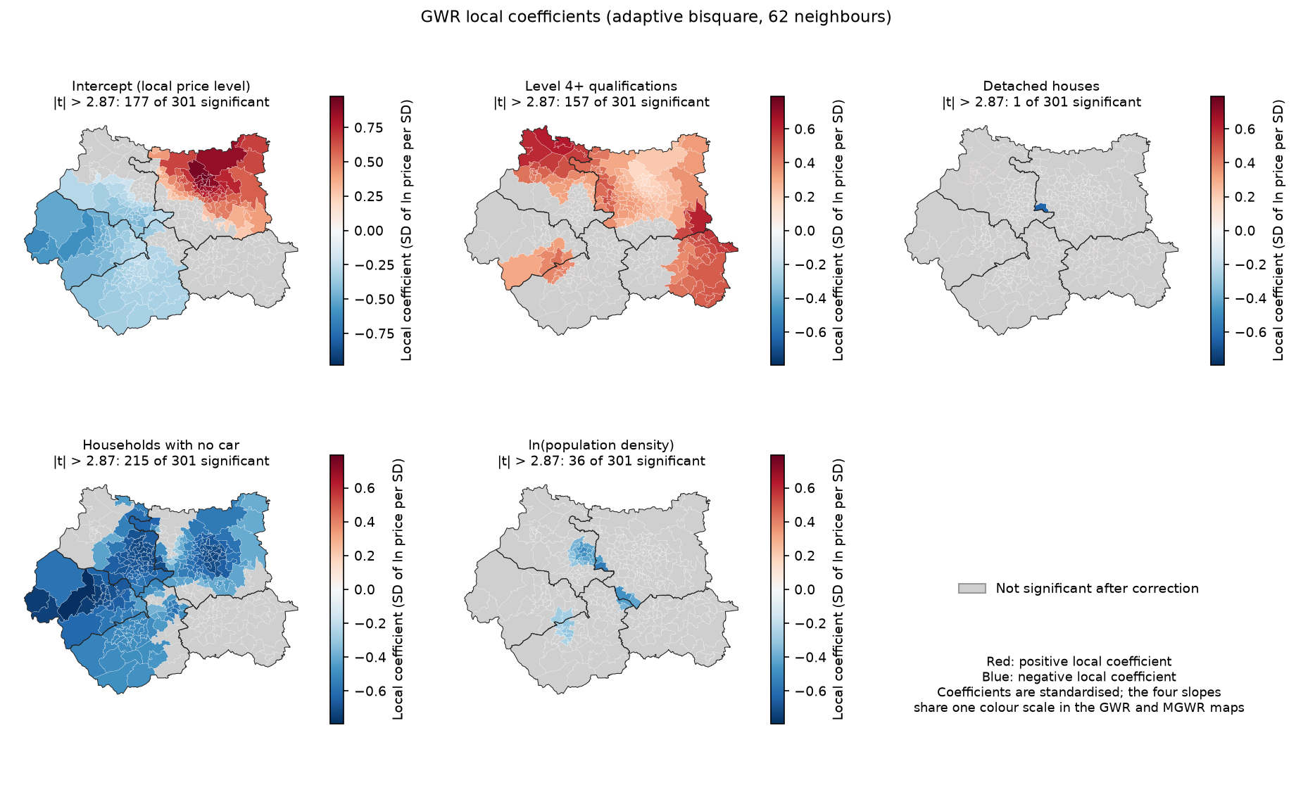
Read with the corrections in mind, the GWR maps suggest:
- The intercept is the strongest local signal. After allowing for the four census variables, prices are higher than average across north and east Leeds and lower in Calderdale, Kirklees and west Bradford. This is the regional price surface that the spatial error model in Part 1 absorbed into its error term.
- Level 4+ qualifications have a positive effect wherever they are significant, apparently strongest in the north of Bradford district and on the eastern side of the county.
- No-car households have a negative effect across the west and centre, but it is not significant in much of Leeds and Wakefield.
- Detached houses and density have little local signal.
How much of that variation is real? GWR uses one bandwidth for every variable, so if the intercept genuinely varies over short distances, every other coefficient is forced to vary over the same distance too. That is the problem MGWR solves.
Step 4: fit MGWR, one bandwidth per variable
Multiscale GWR (Fotheringham, Yang and Kang, 2017) lets each variable have its own bandwidth. A variable whose effect really is constant gets a bandwidth near n, which makes it effectively global, while a variable that varies locally gets a small one. It is fitted by back-fitting, which cycles through the variables and re-optimises each bandwidth until the estimates converge. That makes it much slower.
t0 = time.perf_counter()mgwr_selector = Sel_BW(coords, y, X, multi=True)mgwr_bws = mgwr_selector.search(criterion="AICc")mgwr = MGWR(coords, y, X, mgwr_selector).fit()print(f"search + fit {time.perf_counter() - t0:.1f} s")mgwr.summary()bw_ci = mgwr.get_bws_intervals(mgwr_selector) # 95% intervals for each bandwidthcrit_j = mgwr.critical_tval() # one corrected critical value per covariatemt_filt = mgwr.filter_tvals()bandwidth search 110.7 s; search + fit 111.7 s (GWR search took 5.0 s)MGWR bandwidths---------------------------------------------------------------------------Variable Bandwidth ENP_j Adj t-val(95%) Adj alpha(95%)X0 54.000 13.675 2.929 0.004X1 298.000 1.373 2.102 0.036X2 300.000 1.340 2.092 0.037X3 300.000 1.203 2.047 0.042X4 43.000 20.053 3.050 0.002
Diagnostic information---------------------------------------------------------------------------Residual sum of squares: 30.090Effective number of parameters (trace(S)): 37.645AICc: 250.042R2 0.900Adjusted R2 0.886
Intercept bandwidth 54 (95% interval 51-65) ENP_j 13.7 critical |t| 2.93 | beta min -0.516 median -0.047 max +0.773 | significant 188 (92 +, 96 -)level4 bandwidth 298 (95% interval 202-298) ENP_j 1.4 critical |t| 2.10 | beta min +0.247 median +0.259 max +0.278 | significant 301 (301 +, 0 -)detached bandwidth 300 (95% interval 240-300) ENP_j 1.3 critical |t| 2.09 | beta min +0.090 median +0.103 max +0.119 | significant 301 (301 +, 0 -)no_car bandwidth 300 (95% interval 240-300) ENP_j 1.2 critical |t| 2.05 | beta min -0.516 median -0.506 max -0.489 | significant 301 (0 +, 301 -)ln_density bandwidth 43 (95% interval 43-57) ENP_j 20.1 critical |t| 3.05 | beta min -0.445 median -0.088 max +0.161 | significant 83 (0 +, 83 -)This is the most informative result in the series. MGWR splits the variables into two groups:
- Local: the intercept (bandwidth 54) and population density (43). These vary over distances of a few kilometres.
- Effectively global: Level 4+ qualifications (298), detached houses (300) and no-car households (300). Their bandwidths are at or next to the maximum of n − 1 = 300 neighbours, and their 95% intervals (202–300 and 240–300) exclude anything as local as GWR’s 62. Their coefficients barely vary:
level4runs only from 0.247 to 0.278.
Much of the variation in the GWR coefficient maps, then, was the single bandwidth forcing every variable to be as local as the intercept. MGWR also needs fewer effective parameters (37.6 against 56.5), so its AICc is much lower (250.0 against 282.1), with almost the same R² (0.900). Each covariate also gets its own corrected critical t-value, from 2.05 for the near-global variables to 3.05 for density, because the correction depends on that covariate’s own ENP_j.
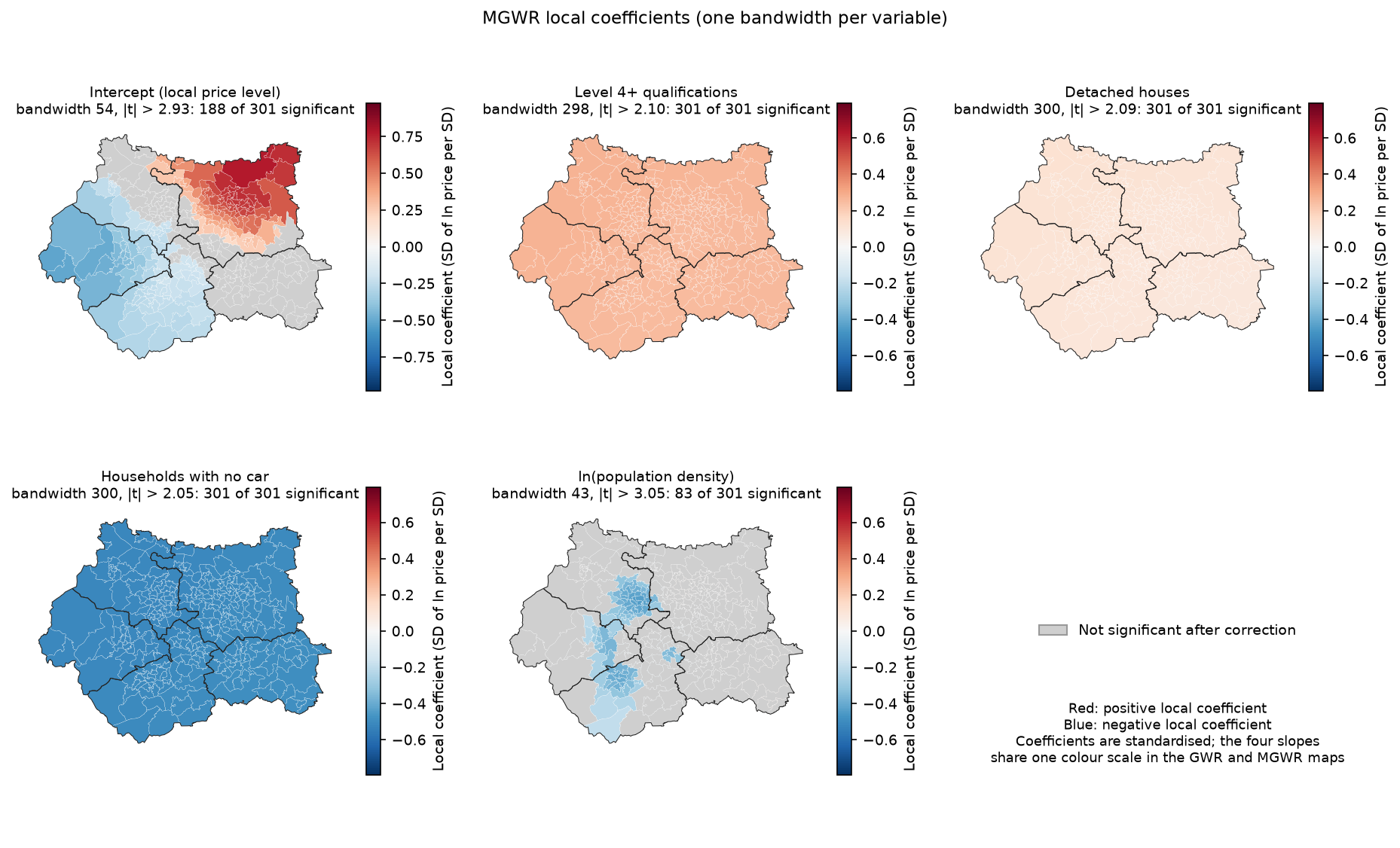
The MGWR global coefficients also agree with Part 1’s spatial error model rather than OLS. The level4 coefficient is about 0.26 SD per SD in MGWR and 0.23 in the error model, against 0.49 in OLS. Both local and global spatial models say the same thing: OLS overstates the qualifications effect because graduates are concentrated in the expensive parts of the county, and once the regional price level is allowed for, the effect roughly halves.
The density effect is new. It is negative and significant in a band from Bradford through Calderdale into Kirklees, where denser MSOAs are cheaper than their other characteristics suggest, and not significant elsewhere. That is a hypothesis worth investigating, perhaps about the type of dense housing in the mill towns compared with central Leeds, not a finding.
Step 5: local R² and local multicollinearity
GWR also gives a local R² for each regression: how well the local model fits the MSOAs around each point.
gdf["gwr_r2"] = gwr.localR2.flatten()corr, vifs, cn, vdp = gwr.local_collinearity() # local correlations, VIFs, condition numbers, VDPsgdf["gwr_cn"] = cn.flatten()mcn, mvdp = mgwr.local_collinearity() # MGWR returns condition numbers and VDPs onlyGWR local R2: min 0.69, median 0.86, max 0.95; global GWR R2 0.907, MGWR R2 0.900lowest local R2: Farnley East (Leeds) 0.69; Holbeck (Leeds) 0.70; Farnley West & Gamble Hill (Leeds) 0.71GWR local condition number: min 3.0, median 5.7, max 18.4; > 30 in 0 MSOAsGWR local VIF max per variable: level4 3.7, detached 13.0, no_car 7.1, ln_density 5.2; MSOAs with any VIF > 10: 4strongest local correlation: detached vs no_car, from -0.92 to -0.65 (global -0.78)MGWR local condition number: median 3.4, max 5.8; > 30 in 0 MSOAs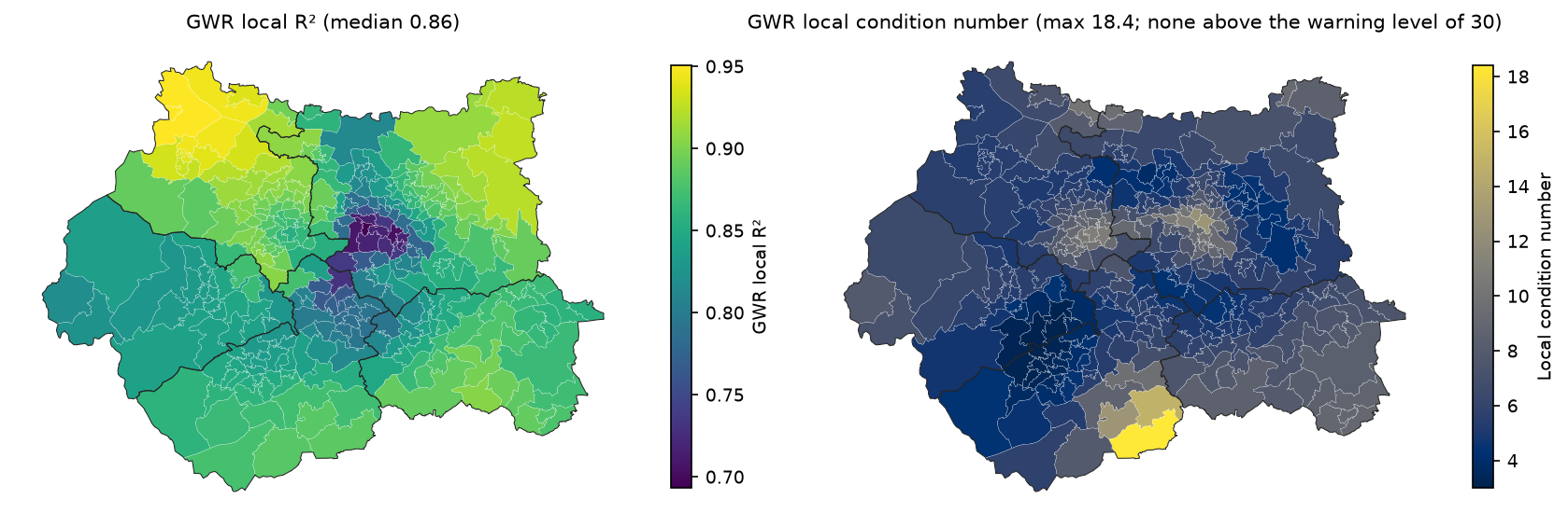
Local R² ranges from 0.69 to 0.95. The model fits best in the north of Bradford district and north-east Leeds, and worst in inner south Leeds (Holbeck and Farnley), where something the four census variables do not capture, perhaps the mix of regeneration and older terraces, drives prices. Low local R² is a pointer to missing variables, not a significance test.
Local multicollinearity is a well-known weakness of GWR (Wheeler and Tiefelsdorf, 2005). Two variables can be only moderately correlated across the whole study area but almost collinear within one local window, and then their local coefficients become unstable and often take opposite, offsetting signs. Here, detached and no_car have a global correlation of −0.78, but locally it reaches −0.92. A few MSOAs have a local VIF above 10, and the local condition numbers, at most 18.4, stay below the usual warning level of 30. So collinearity is not driving the results, but it is a plausible contributor to the wide, insignificant swings in GWR’s detached coefficient (−0.64 to +0.54), since detached is the variable with the highest local VIF. MGWR, whose condition numbers are at most 5.8, does not show the problem.
Step 6: compare with the global models from Part 1
model R2 AICc resid_I resid_p ENP OLS 0.739 462.041 0.457 0.000 5.000 Spatial lag (ML) 0.848 319.916 0.094 0.003 6.000Spatial error (ML) 0.696 301.679 -0.074 0.016 6.000 GWR (bw 62) 0.907 282.094 -0.027 0.254 56.517 MGWR 0.900 250.042 -0.034 0.189 37.645The R² of the lag model is spreg’s pseudo R², and the R² of the error model covers only its non-spatial part, so compare the models by AICc, not R².
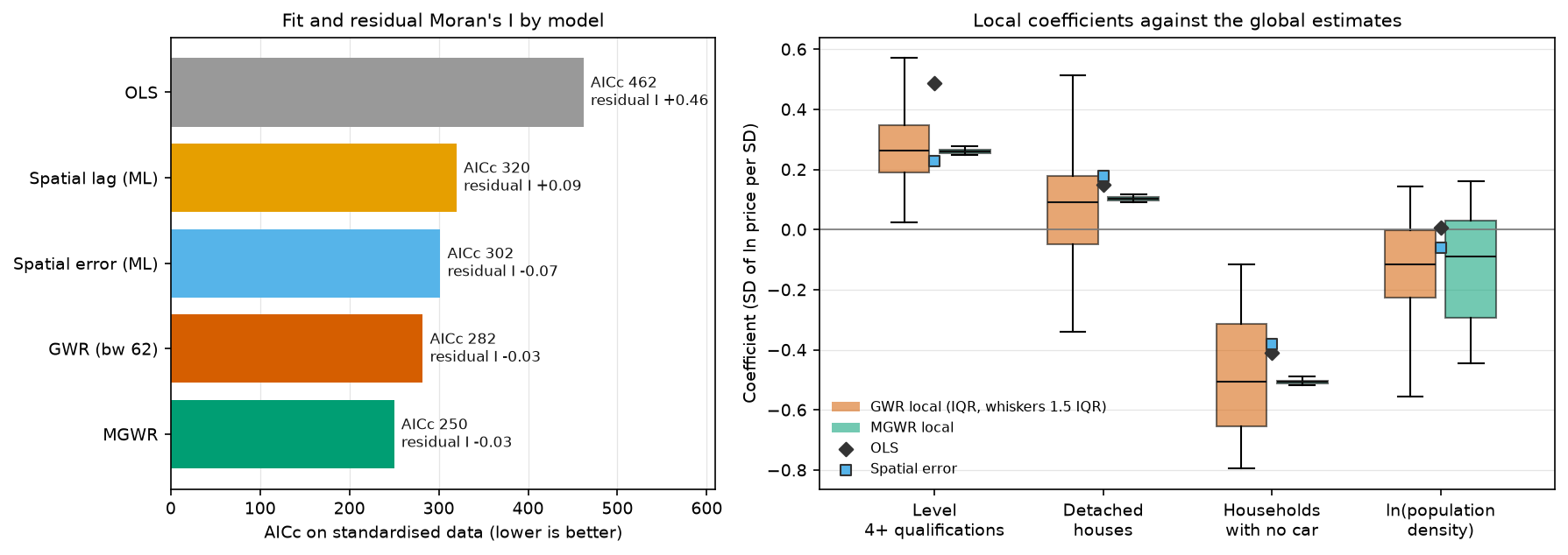
By AICc the order is MGWR < GWR < spatial error < spatial lag < OLS. Both local models remove the residual spatial autocorrelation altogether (I = −0.03, p ≈ 0.2), which neither global spatial model quite managed. The box plots show the other side of the trade-off: GWR’s local estimates spread widely around the global values, while MGWR collapses three of the four back to a single global value.
What should you report? MGWR is the best-fitting and the most honest about which effects vary. But a mixed model is not always the right deliverable. If the question is “what is the effect of X?”, the spatial error model of Part 1 gives one coefficient with a standard error that respects spatial dependence. If the question is “where does the relationship differ?”, MGWR is the tool, and here its answer is that the relationships with qualifications, housing type and car ownership hardly differ. What differs is the baseline price level.
Pitfalls and limitations
- GWR is exploratory. It is a tool for spotting where a global model may be wrong, not for estimating causal local effects. Local coefficients are smoothed, correlated with their neighbours, and depend on the bandwidth and kernel. Treat patterns as hypotheses to test with better data or a theory-driven model.
- Multiple testing. Hundreds of local t-tests need a correction. Use mgwr’s corrected critical values by calling
filter_tvals()andcritical_tval()withoutalpha. For the formal question “does this coefficient really vary?”, mgwr has a Monte Carlo test,results.spatial_variability(selector, n_iters=1000). It refits the model for each random permutation of the locations, so it is very slow; MGWR’s bandwidth intervals answer much the same question here. - Local multicollinearity. Always check the local condition numbers and VIFs. Values above 30 (condition number) or 10 (VIF) mean the local coefficients in those places should not be interpreted. Here the largest condition number is 18.4, but four MSOAs have a local VIF above 10.
- Computing time. GWR on 301 areas took 5 s to choose the bandwidth; MGWR took 111 s on a laptop (89 s on an earlier run, so expect variation). MGWR scales badly with n because each back-fitting iteration refits n local regressions per variable. For larger data, restrict the bandwidth search (
multi_bw_min,multi_bw_max), start MGWR from the GWR bandwidth (init_multi), and use parallel processing (n_jobsinSel_BW). For tens of thousands of points, consider the FastGWR implementation. - Same data caveats as Part 1. These are associations across 301 areas. The census is from 2021 and the prices from the year to March 2026. MSOA medians are noisy. MSOAs at the edge of West Yorkshire have their local regressions shifted inwards, because the data stop at the county boundary.
- The bandwidth curve is flat. AICc changes by only a few points between about 55 and 90 neighbours. Coefficient maps from bandwidths in that range are equally defensible, so do not over-read fine detail.
Frequently asked questions
What is geographically weighted regression used for?
GWR is used to explore whether the relationship between a dependent variable and its predictors changes across space: for example, whether house prices respond more to schools in one city than another, or whether a disease risk factor matters more in some regions. It produces a map of each coefficient, a local R² and local residuals.
What is the difference between GWR and MGWR?
GWR uses one bandwidth for every variable, so all coefficients vary over the same spatial scale. MGWR gives each variable its own bandwidth, so some can be local, some regional and some global. MGWR usually fits better, is less noisy, and tells you directly which relationships vary, but it is much slower to fit.
How do I choose the bandwidth in GWR?
Let the data choose it by minimising AICc (or cross-validation) with mgwr’s Sel_BW(...).search(criterion="AICc"). Use an adaptive kernel (a number of nearest neighbours) when your areas vary a lot in size, as census areas do. Plot AICc against the bandwidth to see how flat the minimum is.
How do I test whether GWR coefficients are significant?
Compare each local t-value with mgwr’s corrected critical value, which adjusts α for the effective number of independent tests (results.critical_tval() with no arguments, or results.filter_tvals() to set non-significant t-values to zero). Grey out the non-significant areas on the coefficient maps. Do not use 1.96 for hundreds of local tests.
Is GWR better than a spatial lag or spatial error model?
They answer different questions. Spatial lag and error models assume one global relationship and model spatial dependence through the weights matrix; GWR and MGWR allow the relationship itself to vary. GWR often fits better because it is much more flexible, but that flexibility costs effective parameters and interpretability. Here MGWR had the lowest AICc, yet its main finding was that three of the four effects are global.
Can I use GWR for prediction?
Yes: mgwr’s GWR.predict() estimates at new locations using the calibrated bandwidth. But GWR is not designed as a predictive model. For prediction at unsampled locations, compare it with kriging or a machine-learning model, evaluated with spatially blocked cross-validation.
Next steps
- If you skipped it, Part 1: spatial regression in Python covers OLS diagnostics, the Lagrange Multiplier tests, spatial lag and error models, and how to interpret lag-model impacts.
- To test the local residuals or coefficients for clustering, use the local statistics in the hot spot analysis tutorial.
- For a simpler first look at a relationship between two census variables, see bivariate correlation analysis with census and crime data (in ArcGIS Pro).
- To produce the coefficient maps at publication quality, see maps in Python with Matplotlib and Cartopy. The script also writes all the local estimates to
output/gwr_mgwr_results.gpkgfor use in QGIS.
Data and licences
- Median house prices by MSOA (formerly HPSSA dataset 2), year ending March 2026, Office for National Statistics, derived from HM Land Registry Price Paid Data. Open Government Licence v3.0. Contains HM Land Registry data © Crown copyright and database right 2026.
- Census 2021 tables TS067, TS044, TS045 and TS006, Office for National Statistics, via Nomis. Open Government Licence v3.0.
- MSOA (December 2021) boundaries EW BGC V3, ONS Open Geography Portal. Open Government Licence v3.0. Contains OS data © Crown copyright and database right 2026.
References: da Silva, A. R. and Fotheringham, A. S. (2016) The multiple testing issue in geographically weighted regression, Geographical Analysis 48(3); Fotheringham, A. S., Yang, W. and Kang, W. (2017) Multiscale geographically weighted regression (MGWR), Annals of the American Association of Geographers 107(6); Oshan, T. M. et al. (2019) mgwr: a Python implementation of multiscale geographically weighted regression, ISPRS International Journal of Geo-Information 8(6); Wheeler, D. and Tiefelsdorf, M. (2005) Multicollinearity and correlation among local regression coefficients in geographically weighted regression, Journal of Geographical Systems 7(2).
Key terms
- Geographically weighted regression (GWR)
- A local regression that fits a separate weighted least-squares model at each location, giving more weight to nearby observations, so that every coefficient can vary across space.
- Multiscale GWR (MGWR)
- An extension of GWR in which each explanatory variable has its own bandwidth, so some relationships can be local and others regional or global. It is fitted by back-fitting.
- Bandwidth
- The size of the local neighbourhood in GWR: a distance (fixed kernel) or a number of nearest neighbours (adaptive kernel). Small bandwidths give local, noisy estimates; a bandwidth of all observations reproduces a global model.
- AICc
- The Akaike information criterion with a small-sample correction. In GWR it uses the trace of the hat matrix as the number of parameters, and it is the usual criterion for choosing the bandwidth.
- Effective number of parameters (ENP)
- The trace of the GWR hat matrix, which measures how flexible the local model is. It is used in AICc and in the multiple-testing correction for local t-values.
- Local condition number
- The condition number of the weighted design matrix at one location. Values above about 30 warn that local collinearity may make the local coefficients unreliable.
Data for this tutorial
- Nomis · Census 2021 bulk tables TS067, TS044, TS045 and TS006 at MSOA level
- Open Geography Portal · Middle layer Super Output Areas (December 2021) boundaries, generalised and clipped (BGC)
- Median house prices by MSOA (ONS) · Median price paid for all dwellings, year ending March 2026, the dependent variable
Licences and formats for each source are listed in the GIS data sources catalogue.