Spatial regression in Python: OLS diagnostics, spatial lag and spatial error models with spreg
Fit spatial regression models in Python with PySAL's spreg on real West Yorkshire house prices: test the OLS residuals for spatial autocorrelation, read the Lagrange Multiplier diagnostics, fit spatial lag and spatial error models, compare them by AIC and log-likelihood, interpret direct, indirect and total impacts, and check how much the spatial weights matter.
- Level
- Intermediate
- Tested with
- Python 3.12
- Source code
- Download scripts
Key takeaways
- Run OLS first and test its residuals. In spreg, `spreg.OLS(y, X, w=w, spat_diag=True, moran=True)` prints Moran's I of the residuals and all the Lagrange Multiplier tests in one summary.
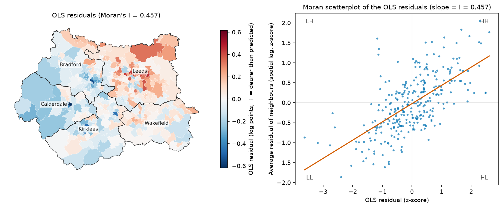
- For median house prices in West Yorkshire's 301 MSOAs, OLS explains 74% of the variation in ln(price), but its residuals are strongly clustered (Moran's I = 0.457, pseudo p = 0.0001). The OLS standard errors are therefore too small.
- Both LM-lag (154.9) and LM-error (168.8) are significant, so look at the robust versions. Robust LM-error (46.0) beats robust LM-lag (32.1) with queen weights and with every KNN weights matrix tried. The spatial error model also has the lower AIC (−364.8 against −344.6).
- A spatial lag coefficient is not a marginal effect. With ρ = 0.528, a 10-point rise in the Level 4+ share everywhere raises prices by 23.7% in total: an 11.3% direct effect plus a spillover of about the same size. OLS says 18.3% and the error model 8.1%.
- The weights matter for the size of the effects, not the story. Across queen, rook and KNN 4–12 weights, λ runs from 0.73 to 0.84 and the lag model's total effect of Level 4+ from 0.020 to 0.027, but the ranking of the models never changes. The spatial Durbin model fits better still.
Before you start
- Comfortable with GeoPandas and with ordinary least squares regression (coefficients, standard errors, R²)
- Global Moran's I and spatial weights at the level of the hot spot analysis tutorial on this site
- Python 3.10+ with geopandas, pyogrio, libpysal, esda, spreg, numpy, pandas, scipy, matplotlib, requests and openpyxl
- An internet connection: the data script downloads about 60 MB of ONS, Nomis and ONS Open Geography files on the first run
Short answer: to run a spatial regression in Python, fit OLS with PySAL’s spreg and pass it a spatial weights matrix: spreg.OLS(y, X, w=w, spat_diag=True, moran=True). If the residuals are spatially autocorrelated, use the Lagrange Multiplier tests in the output to choose a model. Fit a spatial lag model with spreg.ML_Lag when the robust LM-lag test is larger, and a spatial error model with spreg.ML_Error when robust LM-error is larger. Then compare the models by AIC, log-likelihood and residual Moran’s I. For a lag model, report the direct, indirect and total impacts, not the raw coefficients. For house prices in West Yorkshire, the spatial error model wins: the AIC falls from −202.3 (OLS) to −364.8, and residual Moran’s I falls from 0.457 to −0.074.
House prices are a textbook case for spatial regression. Expensive areas sit next to expensive areas, and the census variables we can use to explain prices never capture everything that makes a place desirable. Fit an ordinary regression and the leftover error is mapped in clusters. That breaks the OLS assumption of independent errors, so the standard errors and p-values are wrong, and some coefficients may be biased too.
In this tutorial you will:
- build a dataset of median house prices and Census 2021 variables for West Yorkshire’s 301 MSOAs;
- fit OLS with spreg and test the residuals for spatial autocorrelation with Moran’s I;
- read the LM-lag, LM-error and robust LM diagnostics;
- fit spatial lag and spatial error models by maximum likelihood, plus GM estimators that tolerate heteroskedasticity;
- compare the models by AIC, log-likelihood and residual autocorrelation;
- interpret the lag model’s direct, indirect and total impacts correctly;
- test how much the answer depends on the spatial weights (queen, rook and KNN).
Part 2 of this series uses the same data to ask a different question: do the relationships themselves vary across West Yorkshire? It fits geographically weighted regression (GWR) and multiscale GWR (MGWR), maps the local coefficients, and compares them with the global models from this part.
All outputs below are real results from spatial_regression.py, run in October 2026 with Python 3.12.0, spreg 1.9.1, libpysal 4.15.1, esda 2.10.0, geopandas 1.2.0 and numpy 2.5.4.
The data: house prices and Census 2021 in West Yorkshire
The dependent variable is the median price paid for all dwellings in the year ending March 2026, by 2021 MSOA. The ONS publishes it as Median house prices by MSOA, the successor to the old house price statistics for small areas (HPSSA) dataset 2, from HM Land Registry’s Price Paid Data. Where an MSOA had fewer than five sales, the value is suppressed as [x]. None of West Yorkshire’s 301 MSOAs is suppressed in this edition.
The explanatory variables come from Census 2021 bulk tables on Nomis:
| Variable | Definition | Census table |
|---|---|---|
level4 |
% of residents aged 16+ with a Level 4 qualification or above (degree level) | TS067 |
detached |
% of households living in a detached house | TS044 |
no_car |
% of households with no car or van | TS045 |
ln_density |
natural log of usual residents per km² | TS006 |
These four capture the usual drivers of small-area prices: the education and income of the residents, the housing stock, and how urban the area is. We model ln(price), so a coefficient b means that a one-unit increase in x changes price by about 100 × b per cent (exactly 100 × (e^b − 1)).
The boundaries are the ONS MSOA (December 2021) BGC polygons, downloaded from the ONS Open Geography ArcGIS service in British National Grid. One small module, wy_data.py, downloads all three sources, joins them and caches a GeoPackage. Both parts of this series use it.
PRICE_URL = ("https://www.ons.gov.uk/file?uri=/peoplepopulationandcommunity/housing/datasets/"             "medianhousepricesbymiddlelayersuperoutputarea/yearendingmarch2026/medianpricepaidformsoa.xlsx")PRICE_COL = "Year ending Mar 2026"NOMIS = "https://www.nomisweb.co.uk/output/census/2021/census2021-{t}.zip"MSOA_URL = ("https://services1.arcgis.com/ESMARspQHYMw9BZ9/arcgis/rest/services/"            "Middle_layer_Super_Output_Areas_December_2021_Boundaries_EW_BGC_V3/FeatureServer/0/query")
def build():    DATA.mkdir(exist_ok=True)    # 1. median price paid, all dwellings, by 2021 MSOA (table 1a); "[x]" = fewer than 5 sales    xlsx = download(PRICE_URL, DATA / "medianpricepaidformsoa_ye_mar2026.xlsx")    price = pd.read_excel(xlsx, sheet_name="1a", header=2, usecols=["Local authority code", "Local authority name",                                                                    "MSOA code", "MSOA name", PRICE_COL])    price = price[price["Local authority code"].isin(LADS)].rename(columns={        "Local authority code": "lad_code", "Local authority name": "lad", "MSOA code": "msoa", "MSOA name": "name",        PRICE_COL: "price"})    price["price"] = pd.to_numeric(price.price, errors="coerce")
    # 2. Census 2021 explanatory variables (shares in per cent)    q, acc, car, dens = (nomis_msoa(t) for t in ("ts067", "ts044", "ts045", "ts006"))    census = pd.DataFrame({        "level4": 100 * q["Highest level of qualification: Level 4 qualifications and above"]        / q["Highest level of qualification: Total: All usual residents aged 16 years and over"],        "detached": 100 * acc["Accommodation type: Detached"] / acc["Accommodation type: Total: All households"],        "no_car": 100 * car["Number of cars or vans: No cars or vans in household"]        / car["Number of cars or vans: Total: All households"],        "density": dens["Population Density: Persons per square kilometre; measures: Value"],    })
    # 3. 2021 MSOA boundaries in British National Grid, filtered to the five districts by name    where = " OR ".join(f"MSOA21NM LIKE '{n} %'" for n in LADS.values())    geo = gpd.read_file(download(MSOA_URL, DATA / "msoa2021_west_yorkshire.geojson", where=where,                                 outFields="MSOA21CD,MSOA21NM", outSR=27700, f="geojson"))    geo = geo.set_crs(CRS, allow_override=True).rename(columns={"MSOA21CD": "msoa", "MSOA21NM": "msoa_nm"})
    gdf = geo.merge(price, on="msoa", how="inner").merge(census, left_on="msoa", right_index=True, how="left")    gdf["ln_price"] = np.log(gdf.price)    gdf["ln_density"] = np.log(gdf.density)    ...
The full module, with the download() and nomis_msoa() helpers, is in the code folder. The main script then loads the data:
from wy_data import load_west_yorkshire
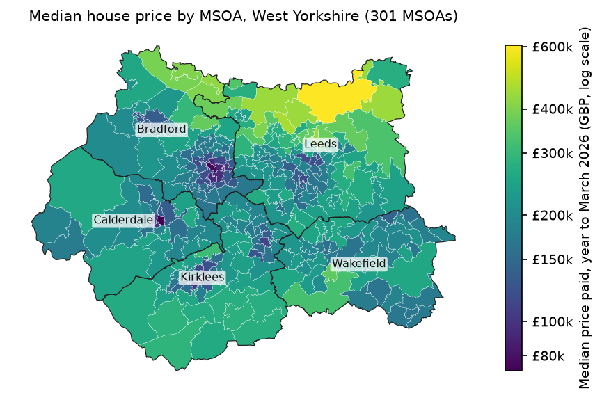
gdf = load_west_yorkshire()X_NAMES = ["level4", "detached", "no_car", "ln_density"]print(gdf[["price", "level4", "detached", "no_car", "density"]].describe().loc[["mean", "min", "50%", "max"]] .round(1).to_string())print("correlations with ln(price): " + ", ".join(f"{c} {gdf.ln_price.corr(gdf[c]):+.2f}" for c in X_NAMES))301 MSOAs with a median price and census data: Leeds 107, Bradford 63, Kirklees 59, Wakefield 45, Calderdale 27 price level4 detached no_car densitymean 215382.2 30.1 17.5 26.1 2987.3min 72500.0 15.1 0.2 7.2 94.150% 202500.0 28.5 14.7 23.2 2512.7max 605000.0 62.8 64.3 66.9 19894.8cheapest: Pellon East (Calderdale) GBP 72,500 | dearest: Collingham, Rigton & Harewood (Leeds) GBP 605,000correlations with ln(price): level4 +0.72, detached +0.68, no_car -0.72, ln_density -0.51Prices range more than eightfold, from £72,500 in Pellon East (Halifax) to £605,000 in Collingham, Rigton & Harewood, north of Leeds. The map shows the pattern we are about to model: an expensive arc across north Leeds, Wharfedale and the Bradford suburbs, and cheaper inner areas in all five towns and cities.
Step 1: build the spatial weights
Every spatial regression needs a spatial weights matrix W that says which MSOAs are neighbours. We start with queen contiguity (MSOAs that share any boundary point) and row-standardise it, so that Wy is the average of the neighbours’ values. The hot spot analysis tutorial explains the main types of weights in more detail. Step 6 below checks whether the choice changes the result.
from libpysal.weights import Queen
w_queen = Queen.from_dataframe(gdf, use_index=False)print(f"queen contiguity: mean {w_queen.mean_neighbors:.2f} neighbours (min {w_queen.min_neighbors}, " f"max {w_queen.max_neighbors}), islands {len(w_queen.islands)}")w_queen.transform = "r" # row-standardisequeen contiguity: mean 5.72 neighbours (min 1, max 12), islands 0There are no islands (MSOAs without neighbours), which matters because spreg’s tests and estimators need every row of W to have at least one neighbour.
Step 2: fit OLS with spatial diagnostics
spreg runs ordinary least squares and, if you pass it w with spat_diag=True and moran=True, adds the spatial diagnostics to the summary. We fit ln(price) on the four census variables:
import spreg
y = gdf[["ln_price"]].to_numpy()   # spreg wants an n x 1 arrayX = gdf[X_NAMES].to_numpy()        # the constant is added for you
ols = spreg.OLS(y, X, w=w_queen, spat_diag=True, moran=True, name_y="ln_price", name_x=X_NAMES, name_w="queen", name_ds="West Yorkshire MSOAs")print(ols.summary)vif = spreg.vif(ols)print("VIF: " + ", ".join(f"{n} {v[0]:.2f}" for n, v in zip(X_NAMES, vif[1:])))R-squared : 0.7391Adjusted R-squared : 0.7356Log likelihood : 106.174 Akaike info criterion : -202.347------------------------------------------------------------------------------------ Variable Coefficient Std.Error t-Statistic Probability------------------------------------------------------------------------------------ CONSTANT 11.92240 0.12372 96.36918 0.00000 level4 0.01679 0.00115 14.62319 0.00000 detached 0.00410 0.00143 2.87367 0.00435 no_car -0.01132 0.00137 -8.27682 0.00000 ln_density 0.00270 0.01388 0.19473 0.84574------------------------------------------------------------------------------------MULTICOLLINEARITY CONDITION NUMBER 33.723Jarque-Bera 2 5.569 0.0618Breusch-Pagan test 4 47.790 0.0000Koenker-Bassett test 4 36.294 0.0000
DIAGNOSTICS FOR SPATIAL DEPENDENCETEST MI/DF VALUE PROBMoran's I (error) 0.4570 13.587 0.0000Lagrange Multiplier (lag) 1 154.879 0.0000Robust LM (lag) 1 32.072 0.0000Lagrange Multiplier (error) 1 168.795 0.0000Robust LM (error) 1 45.988 0.0000Lagrange Multiplier (SARMA) 2 200.867 0.0000VIF: level4 1.26, detached 3.06, no_car 2.76, ln_density 1.91On its face this is a good model. R² is 0.74, and three of the four variables are highly significant with the expected signs. A 1-point rise in the share of residents with Level 4+ qualifications goes with 1.7% higher prices (100 × 0.01679), and a 1-point rise in households without a car with 1.1% lower prices. Once the other three are held constant, density adds nothing (p = 0.85).
Multicollinearity is not a problem here. The largest VIF is 3.06 (detached), and the condition number of 33.7 is only just above the rule-of-thumb warning level of 30, mainly because the variables are not centred. The residuals are close to normal (Jarque-Bera p = 0.06) but clearly heteroskedastic (Breusch-Pagan 47.8, p < 0.0001). Keep that in mind: the maximum likelihood estimators below assume constant variance, so Step 4 checks them against estimators that do not.
Step 3: are the residuals spatially autocorrelated?
The Moran's I (error) line says yes: I = 0.457. spreg’s z-value of 13.6 relies on a normal approximation, so we confirm it with a permutation test in esda and map the residuals. Moran’s I itself, the scatterplot and permutation inference are explained in the hot spot analysis tutorial. Here we just apply it to the residuals.
import esda
np.random.seed(42) # esda.Moran has no seed argumente_ols = ols.u.flatten()mi_ols = esda.Moran(e_ols, w_queen, permutations=9999)print(f"I = {mi_ols.I:.3f} E[I] = {mi_ols.EI:.4f} z(permutation) = {mi_ols.z_sim:.1f} pseudo p = {mi_ols.p_sim:.4f}")print(f"largest of 9999 permuted I values: {mi_ols.sim.max():.3f}")I = 0.457 E[I] = -0.0033 z(permutation) = 13.2 pseudo p = 0.0001largest of 9999 permuted I values: 0.137 Pellon East (Calderdale): residual -0.616 = price -46% vs the OLS fit Central Bradford (Bradford): residual -0.541 = price -42% vs the OLS fit Birkby (Kirklees): residual -0.471 = price -38% vs the OLS fit Dewsbury Central & Westborough (Kirklees): residual -0.456 = price -37% vs the OLS fitNone of the 9,999 random rearrangements came anywhere near 0.457; the largest was 0.137. The residual map shows why. OLS underpredicts prices across north and west Leeds and the Aire and Wharfe valleys (red), and overpredicts them in the inner areas of Bradford, Halifax, Huddersfield and Dewsbury (blue). The model is missing something that varies smoothly in space: perhaps housing quality, school catchments, access to Leeds, or simply the market’s view of each town.
Step 4: choose a model with the Lagrange Multiplier tests
The two classic spatial alternatives to OLS differ in where the spatial dependence sits:
- the spatial lag model (SAR), y = ρWy + Xβ + ε, says that the price in an MSOA depends directly on prices in neighbouring MSOAs. This is a substantive spillover, for example because buyers and valuers compare nearby sales.
- the spatial error model (SEM), y = Xβ + u with u = λWu + ε, says that the errors are clustered, typically because a spatially smooth variable has been left out. The β keep their ordinary meaning.
The LM tests are computed from the OLS residuals and ask whether each extra term would help. The standard decision rule (Anselin, 2005) is:
- If neither LM-lag nor LM-error is significant, keep OLS.
- If only one is significant, fit that model.
- If both are significant, as here, compare the robust versions, each of which tests one alternative while allowing for the other. Fit the model with the larger robust statistic.
Here robust LM-error (46.0) beats robust LM-lag (32.1), so the rule points to the spatial error model. But both robust tests are still highly significant, which hints that both kinds of dependence may be present. spreg also reports the tests for a spatial Durbin model (LM test for WX = 51.3), and we return to it below. In practice, fit both models and compare them.
Step 5: fit the spatial lag and spatial error models
Both models are fitted by maximum likelihood (ML_Lag, ML_Error). Pass spat_impacts="full" to the lag model so that spreg computes the impacts properly (Step 6 explains why).
lag = spreg.ML_Lag(y, X, w=w_queen, name_y="ln_price", name_x=X_NAMES, name_w="queen", spat_impacts="full")print(lag.summary)err = spreg.ML_Error(y, X, w=w_queen, name_y="ln_price", name_x=X_NAMES, name_w="queen")print(err.summary)Pseudo R-squared : 0.8478Log likelihood : 178.2843Sigma-square ML : 0.0169 Akaike info criterion : -344.569 Variable Coefficient Std.Error z-Statistic Probability CONSTANT 5.47883 0.49081 11.16291 0.00000 level4 0.01004 0.00096 10.40825 0.00000 detached 0.00430 0.00108 3.98087 0.00007 no_car -0.00746 0.00110 -6.80945 0.00000 ln_density 0.01291 0.01060 1.21806 0.22320 W_ln_price 0.52841 0.03884 13.60451 0.00000Pseudo R-squared : 0.6956Log likelihood : 187.4028Sigma-square ML : 0.0143 Akaike info criterion : -364.806 Variable Coefficient Std.Error z-Statistic Probability CONSTANT 12.34069 0.12273 100.55231 0.00000 level4 0.00783 0.00131 6.00037 0.00000 detached 0.00491 0.00111 4.43077 0.00001 no_car -0.01056 0.00131 -8.06595 0.00000 ln_density -0.01998 0.01226 -1.62946 0.10322 lambda 0.79614 0.04087 19.47824 0.00000Both spatial parameters are large and very significant: ρ = 0.528 in the lag model and λ = 0.796 in the error model. Do not compare the pseudo R² values across models. The lag model’s includes the part of y predicted by Wy, while the error model’s measures only the non-spatial part Xβ, so it looks lower even though the model fits better.
The most important change is to level4. In the error model its coefficient falls from 0.0168 to 0.0078, less than half the OLS value. Part of what OLS credited to qualifications is really a regional price surface: areas with many graduates tend to sit in the expensive north of the county, and the error term now absorbs that. The coefficients for detached and no_car change much less.
Compare the models
The three models are nested, so we can compare them by log-likelihood, AIC, likelihood-ratio (LR) tests and the autocorrelation left in their residuals. For the lag model, test the residuals lag.u; for the error model, test the spatially filtered residuals err.e_filtered (ε, not u).
from scipy import stats
def resid_moran(e, w):    m = esda.Moran(np.asarray(e).flatten(), w, permutations=9999)    return m.I, m.p_sim
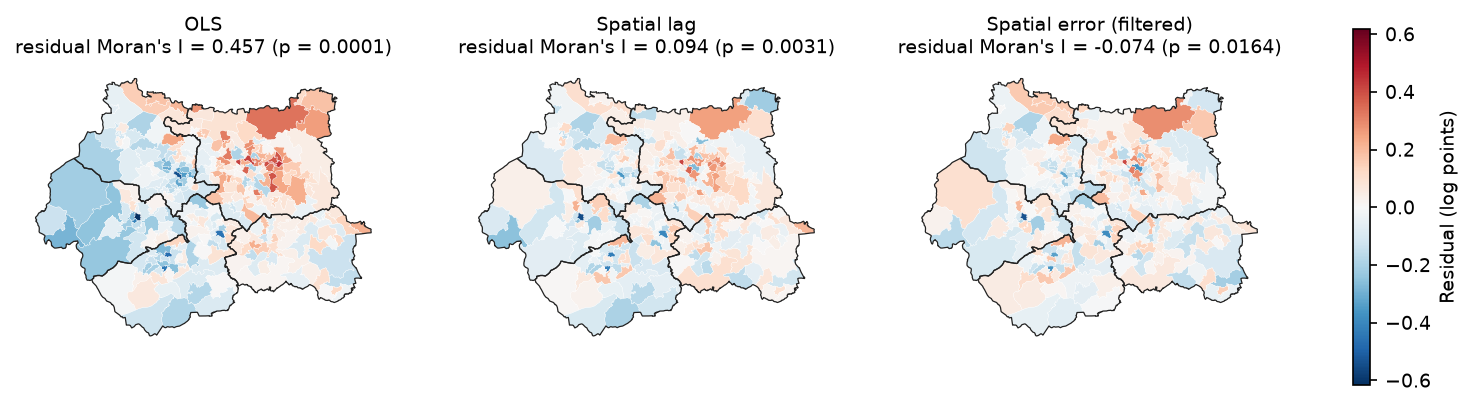
mi_lag = resid_moran(lag.u, w_queen)mi_err = resid_moran(err.e_filtered, w_queen)for name, ll in [("lag vs OLS", lag.logll), ("error vs OLS", err.logll)]: lr = 2 * (ll - ols.logll) print(f"LR {name}: {lr:.1f} (df 1, p = {stats.chi2.sf(lr, 1):.1e})") model logL AIC SC params resid_I resid_p OLS 106.174 -202.347 -183.812 5 0.457 0.000 Spatial lag (ML) 178.284 -344.569 -322.326 6 0.094 0.003 Spatial error (ML) 187.403 -364.806 -346.270 6 -0.074 0.016Spatial Durbin (ML) 201.027 -382.055 -344.984 10 -0.052 0.077LR lag vs OLS: 144.2 (df 1, p = 3.2e-33)LR error vs OLS: 162.5 (df 1, p = 3.3e-37)LR Durbin vs lag: 45.5 (df 4, p = 3.2e-09)LR Durbin vs error (common factor): 27.2 (df 4, p = 1.8e-05)Both spatial models are vast improvements on OLS (LR = 144 and 163 on one degree of freedom). The error model fits better than the lag model: its log-likelihood is higher by 9.1 with the same number of parameters, and its AIC and Schwarz criterion are both lower. This agrees with the robust LM tests.
The lag model still leaves significant positive autocorrelation in its residuals (I = 0.094, p = 0.003). The error model’s filtered residuals are slightly negative (I = −0.074, p = 0.016), which suggests that λ = 0.80 may over-smooth a little. Neither is perfect. That is why the table includes a fourth model.
The spatial Durbin model (SDM, ML_Lag(..., slx_lags=1)) adds the neighbours’ averages WX of all four variables to the lag model. It has the best AIC (−382.1), leaves the least residual autocorrelation (I = −0.052, p = 0.08), and beats both simpler models in LR tests. The “common factor” test (LR = 27.2, df 4) rejects the restriction that would reduce it to the error model. Its main new term is a negative W_detached (−0.0063, p = 0.0008): an MSOA is dearer when it has many detached houses, but slightly cheaper when its neighbours have many. One reading is that a high-detached area surrounded by other high-detached areas is a rural fringe, while one surrounded by terraces is a premium suburb.
The lesson is not that you must always fit an SDM. It is that the LM tests choose between two restricted models, and a model that nests both is worth checking before you settle on one.
Heteroskedasticity: check with GM estimators
The ML estimators assume homoskedastic errors, and the Breusch-Pagan test rejected that. spreg has generalised method of moments (GM) estimators that do not need the assumption: GM_Error_Het for the error model, and GM_Lag with White standard errors for the lag model.
gm_err = spreg.GM_Error_Het(y, X, w=w_queen, name_y="ln_price", name_x=X_NAMES)gm_lag = spreg.GM_Lag(y, X, w=w_queen, robust="white", name_y="ln_price", name_x=X_NAMES)level4 GM error (het) +0.0099 (z +6.1) GM lag (White) +0.0117 (z +10.6)detached GM error (het) +0.0043 (z +3.8) GM lag (White) +0.0042 (z +4.2)no_car GM error (het) -0.0110 (z -6.0) GM lag (White) -0.0084 (z -6.2)ln_density GM error (het) -0.0161 (z -1.5) GM lag (White) +0.0104 (z +1.0)GM error lambda 0.761 | GM lag rho 0.397The signs and significance are unchanged. The GM error model gives a slightly larger level4 effect (0.0099 against 0.0078) and a slightly smaller λ (0.761). The GM lag estimate of ρ is noticeably lower (0.397 against 0.528), because it uses spatially lagged X as instruments rather than the full likelihood. The substantive conclusions survive, but it is a reminder that ρ is estimated with real uncertainty.
Step 6: interpret the spatial lag model’s impacts
This is the step most often done wrongly. In the lag model, β is not the marginal effect of x. Because y appears on both sides, y = (I − ρW)⁻¹(Xβ + ε). A change in x in one MSOA changes its own price, which changes its neighbours’ prices through ρW, which feeds back to the first MSOA, and so on. LeSage and Pace (2009) summarise the n × n matrix of effects with three numbers per variable:
- the direct impact: the average effect of a change in x_i on y_i, including the feedback through the neighbours. It is β × mean(diag((I − ρW)⁻¹)).
- the indirect impact (spillover): the average effect on all other MSOAs combined.
- the total impact: their sum, β / (1 − ρ). This is the effect of a change in x in every MSOA at once.
spreg prints all three with spat_impacts="full". Use "full" or "power", not "simple", which reports direct = β and so ignores the feedback. spreg gives no confidence intervals, so the script simulates them: it draws (β, ρ) 2,000 times from their estimated sampling distribution and recomputes the impacts with the eigenvalues of W.
def lag_impacts(betas, rho, eig):    """Direct, indirect and total impacts of a spatial lag model, from the eigenvalues of W."""    m_dir = np.mean(1.0 / (1.0 - rho * eig)).real    direct = betas * m_dir    total = betas / (1.0 - rho)    return direct, total - direct, total
def lag_impact_ci(model, eig, draws=2000):    params = model.betas.flatten()   # constant, x..., rho    k = len(X_NAMES)    point = lag_impacts(params[1:1 + k], params[-1], eig)    sims = rng.multivariate_normal(params, model.vm, size=draws)    sims = sims[np.abs(sims[:, -1]) < 1]    s = np.array([lag_impacts(d[1:1 + k], d[-1], eig) for d in sims])    return point, np.percentile(s, 2.5, axis=0), np.percentile(s, 97.5, axis=0)
eig_q = np.linalg.eigvals(w_queen.full()[0])(dir_, ind_, tot_), lo_i, hi_i = lag_impact_ci(lag, eig_q)SPATIAL LAG MODEL IMPACTSImpacts computed using the 'full' method. Variable Direct Indirect Total level4 0.0107 0.0106 0.0213 detached 0.0046 0.0045 0.0091 no_car -0.0080 -0.0079 -0.0158 ln_density 0.0138 0.0136 0.0274
rho = 0.528; spatial multiplier 1/(1-rho) = 2.12level4 direct +0.0107 [+0.0089, +0.0127] indirect +0.0106 [+0.0081, +0.0139] total +0.0213 [+0.0178, +0.0256]detached direct +0.0046 [+0.0022, +0.0069] indirect +0.0045 [+0.0020, +0.0075] total +0.0091 [+0.0044, +0.0142]no_car direct -0.0080 [-0.0102, -0.0056] indirect -0.0079 [-0.0108, -0.0054] total -0.0158 [-0.0202, -0.0114]ln_density direct +0.0138 [-0.0083, +0.0371] indirect +0.0136 [-0.0077, +0.0399] total +0.0274 [-0.0159, +0.0759]level4: +10 percentage points everywhere -> total +23.7% on prices (direct +11.3%); OLS said +18.3%My simulated point estimates match spreg’s exactly, which is a useful check. Here is how to read the level4 row:
- The direct impact (0.0107) is a little larger than β (0.0100). The difference is the feedback: a rise in one MSOA’s price raises its neighbours’ prices, which raises its own again.
- The indirect impact (0.0106) is almost as large as the direct one. Raising the graduate share in one MSOA is associated with higher prices in the MSOAs around it.
- The total impact (0.0213) is β times the spatial multiplier 1 / (1 − 0.528) = 2.12. If the Level 4+ share rose by 10 points in every MSOA, the model predicts prices about 23.7% higher (100 × (e^0.213 − 1)). OLS says 18.3%.
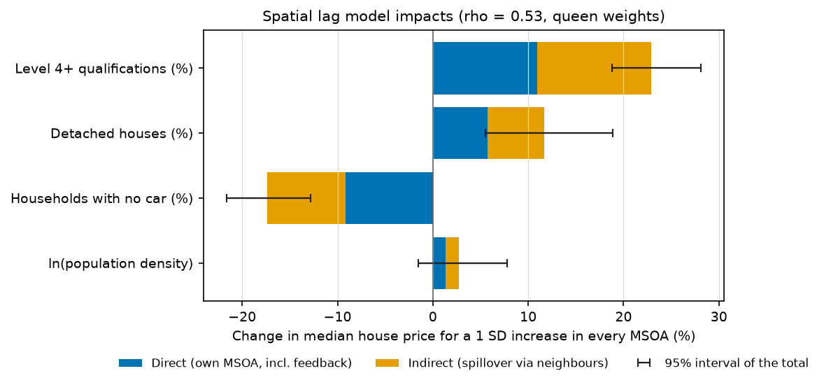
Two cautions. First, in a pure lag model the ratio of indirect to direct impact is the same for every variable: here it is 0.99 for all four. That ratio comes from ρ and W, not from the data on each variable, so the model cannot tell you that one variable spills over more than another. The spatial Durbin model can: its total impact for detached is −0.002, because the negative W_detached term cancels the positive direct effect.
Second, these are equilibrium effects of a change applied everywhere, and they come from a cross-section. They describe how prices and census characteristics co-vary across space, not what would happen if a policy raised qualification levels.
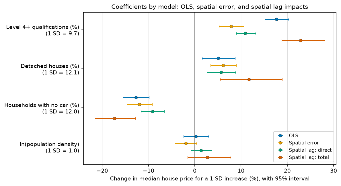
The coefficient chart puts the models side by side on one scale: the % change in price for a one-standard-deviation increase in each variable. The error model’s level4 effect (+7.9% per SD) is less than half of OLS’s (+17.7%). The lag model’s direct effect (+10.9%) sits in between, and its total (+22.9%) is the largest. Which number you report depends on which model you believe, and on whether you mean the effect in one area or everywhere.
Step 7: how sensitive is the result to the weights?
Queen contiguity is a convention, not a fact. Rural MSOAs are large and have few neighbours, while inner-city ones are small and have many, so contiguity weights mean different distances in different places. k-nearest-neighbour (KNN) weights give every MSOA the same number of neighbours. The script refits everything with rook contiguity and with KNN weights for k = 4, 6, 8 and 12, using representative points inside each polygon.
import libpysalfrom libpysal.weights import KNN
cents = gdf.copy(); cents["geometry"] = gdf.representative_point()weights = {"queen": w_queen, "rook": libpysal.weights.Rook.from_dataframe(gdf, use_index=False)}for k in (4, 6, 8, 12): weights[f"knn{k}"] = KNN.from_dataframe(cents, k=k, use_index=False)for name, w in weights.items(): w.transform = "r" o = spreg.OLS(y, X, w=w, spat_diag=True, moran=True) lg = spreg.ML_Lag(y, X, w=w) er = spreg.ML_Error(y, X, w=w) ...weights mean_nbrs resid_I rLM_lag rLM_err rho lambda AIC_lag AIC_err lag_total_level4 err_level4 queen 5.7209 0.4570 32.0719 45.9879 0.5284 0.7961 -344.5687 -364.8056 0.0213 0.0078 rook 5.7076 0.4579 32.5057 45.6931 0.5298 0.7979 -345.7827 -366.2278 0.0213 0.0077 knn4 4.0000 0.4982 21.2865 56.1741 0.4816 0.7340 -330.1602 -354.6328 0.0200 0.0083 knn6 6.0000 0.4783 27.1228 89.9285 0.5048 0.7678 -336.1765 -363.2644 0.0215 0.0084 knn8 8.0000 0.4595 33.4480 121.8362 0.5443 0.7980 -347.4367 -369.1153 0.0234 0.0085 knn12 12.0000 0.4460 30.4394 217.6643 0.5749 0.8417 -346.5446 -380.4566 0.0268 0.0085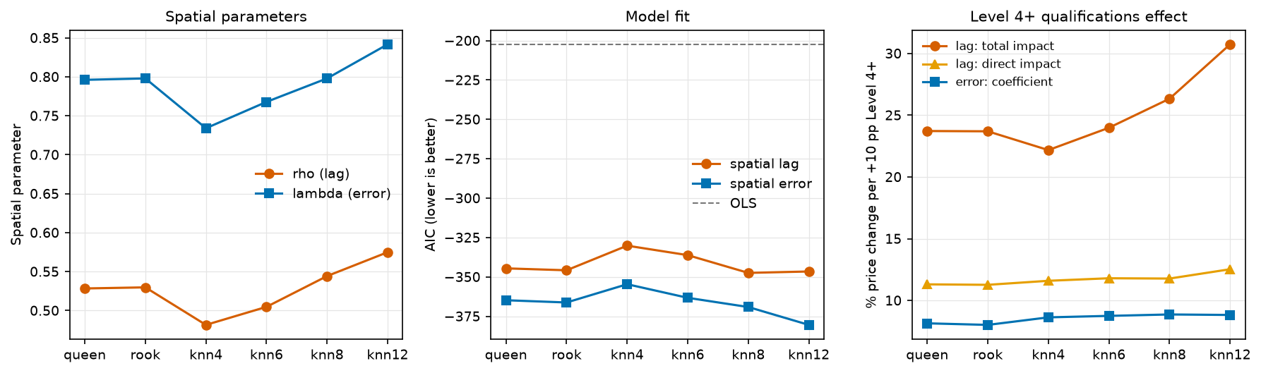
Three things hold for every matrix:
- the OLS residuals are strongly autocorrelated (I = 0.45 to 0.50);
- robust LM-error exceeds robust LM-lag, and the error model has the lower AIC;
- the error model’s
level4coefficient stays between 0.0077 and 0.0085.
The size of the spatial effects does depend on W. With more neighbours each MSOA’s lag is a smoother regional average, ρ and λ rise, and the lag model’s total level4 impact grows from 0.0200 (KNN 4) to 0.0268 (KNN 12): from +22% to +31% for a 10-point rise. The direct impact barely moves (0.0107 to 0.0118), so the extra comes almost entirely from the spillover. If you report spillovers from a lag model, report how they depend on W.
AIC is lowest for KNN 12, but treat cross-W comparisons of AIC as a guide only. Choose the weights for a substantive reason (how far do buyers search, what counts as a neighbourhood?) and then show that the conclusions survive the alternatives, as here.
Limitations and honest caveats
- Association, not causation. These are cross-sectional models of 301 areas. A graduate share does not cause high prices; both reflect income, jobs, schools and housing quality that the model does not measure. The spatial terms soak up some of that omitted structure but do not identify causal effects.
- Ecological fallacy and MAUP. The results describe MSOAs, not households, and they could change with a different set of areas (LSOAs, wards). The modifiable areal unit problem applies to regression just as it does to clustering.
- A time mismatch. The census describes March 2021; the prices are for sales in the year to March 2026. Small areas change slowly, but new-build estates in particular can shift both.
- Medians from small samples. Each median rests on one year’s sales in an area of a few thousand households, so it is noisy, and MSOAs with fewer than five sales are suppressed altogether. Prices also mix flats, terraces and detached houses, so part of the
detachedeffect is simply that detached houses cost more. - Edge effects. MSOAs on the West Yorkshire boundary have neighbours in North Yorkshire, Greater Manchester, Lancashire, South Yorkshire and Derbyshire that are not in the data, so their spatial lags are averages of fewer, inward-facing neighbours.
- Heteroskedasticity. The ML models assume constant error variance, which the Breusch-Pagan test rejects. The GM estimators give similar answers, but the ML standard errors should be treated as approximate.
- Model choice depends on W. The LM tests and AIC compare models for a given W. Here the ranking was stable, but that will not always be true.
Frequently asked questions
What is the difference between a spatial lag and a spatial error model?
A spatial lag model puts the neighbours’ outcome Wy on the right-hand side, so it models a real spillover: prices in one area depend on prices next door. A spatial error model keeps the ordinary regression but lets the errors be correlated across neighbours, which treats spatial dependence as a nuisance caused by clustered omitted variables. The lag model’s coefficients need converting to impacts; the error model’s coefficients can be read like OLS coefficients.
How do I choose between the spatial lag and spatial error model?
Fit OLS with spat_diag=True and read the Lagrange Multiplier tests. If only LM-lag or only LM-error is significant, fit that model. If both are, compare the robust LM tests and pick the larger. Then confirm the choice with log-likelihood, AIC and the Moran’s I of each model’s residuals, and consider a spatial Durbin model, which nests the lag model and, with a restriction, the error model.
How do I interpret the coefficients of a spatial lag model?
Not directly. Report the direct, indirect and total impacts, which spreg prints when you pass spat_impacts="full". The total impact is β / (1 − ρ), the effect of changing x in every area. The direct impact is the average effect of an area’s own x on its own y, including feedback. The indirect impact is the spillover to everyone else.
Should I use ML or GM estimation in spreg?
ML (ML_Lag, ML_Error) is efficient when the errors are normal and homoskedastic, and it gives a log-likelihood and AIC for model comparison. GM estimators (GM_Lag, GM_Error_Het) are faster on large datasets and robust to heteroskedasticity, but have no likelihood. A good routine is to use ML for model comparison and GM as a robustness check when the Breusch-Pagan test is significant.
Do I need spatial regression if Moran’s I of my variables is high?
Not necessarily. What matters is autocorrelation in the residuals of your model, not in the raw variables. If the explanatory variables capture the spatial pattern, the residuals may be random and OLS is fine. Always test the residuals; that is the check this tutorial starts with.
Which spatial weights should I use for regression?
There is no single right answer. Queen contiguity is the usual default for areal data; KNN weights give every area the same number of neighbours and avoid islands; distance bands suit point data. Choose W for a substantive reason, row-standardise it, and refit with one or two alternatives to show how much the results depend on it, as in Step 7.
Next steps
- Part 2: geographically weighted regression in Python fits GWR and MGWR to the same data to ask whether the relationships themselves vary across West Yorkshire, and compares them with the global models here.
- For the full treatment of Moran’s I, LISA and Getis-Ord Gi*, see the hot spot analysis tutorial.
- For a simpler introduction to relating two census variables, see bivariate correlation analysis with census and crime data (in ArcGIS Pro).
- To attach other area-level data to MSOAs, see spatial joins with GeoPandas, and for publication-quality choropleths, maps in Python with Matplotlib and Cartopy.
- If you need predictions at unsampled points rather than area-level effects, kriging is the geostatistical alternative.
Data and licences
- Median house prices by MSOA (formerly HPSSA dataset 2), year ending March 2026, Office for National Statistics, derived from HM Land Registry Price Paid Data. Open Government Licence v3.0. Contains HM Land Registry data © Crown copyright and database right 2026.
- Census 2021 tables TS067, TS044, TS045 and TS006, Office for National Statistics, via Nomis. Open Government Licence v3.0.
- MSOA (December 2021) boundaries EW BGC V3, ONS Open Geography Portal. Open Government Licence v3.0. Contains OS data © Crown copyright and database right 2026.
References: Anselin, L. (2005) Exploring Spatial Data with GeoDa: A Workbook, on the LM decision rule; LeSage, J. and Pace, R. K. (2009) Introduction to Spatial Econometrics, CRC Press, on impacts.
Key terms
- Spatial lag model (SAR)
- A regression with the spatially lagged dependent variable Wy on the right-hand side: y = ρWy + Xβ + ε. It models spillovers, where the outcome in one area depends on the outcome in its neighbours.
- Spatial error model (SEM)
- A regression whose errors are spatially autocorrelated: y = Xβ + u, u = λWu + ε. It models omitted variables that are themselves clustered in space; the β keep their usual meaning.
- Lagrange Multiplier (LM) tests
- Tests computed from the OLS residuals that ask whether adding a spatial lag (LM-lag) or a spatial error term (LM-error) would improve the model. The robust versions test each one while allowing for the other.
- Direct, indirect and total impacts
- In a spatial lag model, the effect of changing x everywhere. The direct impact is the average effect on the area's own y, including feedback through its neighbours. The indirect impact is the spillover to other areas, and the total is their sum, β / (1 − ρ).
- Spatial weights matrix (W)
- An n × n matrix that says which areas are neighbours, for example shared boundaries (queen contiguity) or the k nearest centroids (KNN). Row-standardised so each row sums to 1, Wy is the average of the neighbours.
- MSOA
- Middle layer Super Output Area: a census reporting area in England and Wales with about 5,000 to 15,000 residents. West Yorkshire has 301 of them in the 2021 geography.
- AIC
- Akaike information criterion: −2 × log-likelihood + 2 × number of parameters. Lower is better. It compares models fitted to the same data by maximum likelihood.
Data for this tutorial
- Nomis · Census 2021 bulk tables TS067 (qualifications), TS044 (accommodation type), TS045 (car or van availability) and TS006 (population density) at MSOA level
- Open Geography Portal · Middle layer Super Output Areas (December 2021) boundaries, generalised and clipped (BGC)
- Median house prices by MSOA (ONS) · Median price paid for all dwellings, year ending March 2026, the dependent variable
Licences and formats for each source are listed in the GIS data sources catalogue.