Two-step floating catchment area (2SFCA) in Python: spatial access to GP practices in Cornwall
Measure spatial accessibility to GP practices in Python with the two-step floating catchment area (2SFCA) method and its distance-decay version (E2SFCA). Build OSMnx drive times for Cornwall from OpenStreetMap, use NHS GP workforce data and Census 2021 population, compare the PySAL access package with a vectorised NumPy version, and test the catchment threshold, the decay function and edge effects.
- Level
- Intermediate
- Tested with
- Python 3.12
- Source code
- Download scripts
Key takeaways
- The two-step floating catchment area (2SFCA) method measures access as supply per head that each place can reach. Step 1 divides each GP practice's GP FTE by the population within its catchment; step 2 sums those ratios for every practice a neighbourhood can reach. The PySAL access package does both steps from three tables: demand, supply and travel costs.
- In Cornwall, 97.3% of residents live within a 10-minute free-flow drive of a GP practice. But the 2SFCA score varies more than twofold: E2SFCA ranges from 0.43 to 0.94 GP FTE per 1,000 residents between the 10th and 90th percentiles of output areas, against a county figure of 0.72.
- Nearness and access are not the same thing. The rank correlation between the drive time to the nearest practice and E2SFCA is only −0.22, because a practice next door can still be stretched over a large population.
- The catchment threshold changes the map. Moving from 30 to 20 minutes keeps the ranking (Spearman 0.77); moving to 10 minutes leaves 2.7% of residents with no practice in reach and the ranking barely matches (0.19). Choose and report the threshold, and test it.
- Include supply and demand beyond the study area. Leaving out Devon and Plymouth changes scores within 10 km of the border by −48% to +80%; adding the Plymouth practices without their patients inflates them by up to 24 times.
Before you start
- Comfortable with GeoPandas and OSMnx basics (see the OSMnx street network tutorial)
- Python 3.10+ with access, osmnx, osmium, geopandas, scipy, pyarrow, matplotlib and requests
- An internet connection: the first run downloads about 105 MB of open data from NHS England, the ONS, Nomis, postcodes.io and Geofabrik, and takes about 3 minutes
Short answer: the two-step floating catchment area (2SFCA) method scores each neighbourhood by the supply per head it can reach. In Python, build a travel-time table from neighbourhoods to facilities (here with OSMnx and a SciPy shortest-path search), then pass demand, supply and costs to the PySAL access package:
from access import Access, weightsA = Access(demand_df=oas, demand_index="OA21CD", demand_value="pop", supply_df=practices, supply_index="PRACTICE_CODE", supply_value="TOTAL_GP_FTE", cost_df=times, cost_origin="origin", cost_dest="dest", cost_name="minutes")A.two_stage_fca(name="2sfca", max_cost=30) # 2SFCAA.enhanced_two_stage_fca(name="e2sfca", max_cost=30, weight_fn=weights.step_fn({10: 1, 20: 0.68, 30: 0.22})) # E2SFCAFor GP practices in Cornwall this gives 0.72 GP FTE per 1,000 residents across the county, but 0.43 to 0.94 between the 10th and 90th percentiles of output areas, with the lowest access around Torpoint and the Rame peninsula, Looe, Padstow, the Lizard and the Roseland, and the highest around Camborne, Redruth and Truro. That is true even though 97.3% of residents live within a 10-minute drive of a practice.
Distance to the nearest GP is easy to measure, but it misses half the story. A village with a surgery round the corner can still struggle for appointments if that surgery has two GPs for 15,000 patients. Floating catchment methods combine the two halves, how far and how much for how many, into a single score that health planners and researchers use to find under-served areas.
This is Part 1 of the series Healthcare accessibility analysis in Python. It measures how good access to GPs is now. Part 2, location-allocation in Python, reuses the same Cornwall road network and asks where new services should go, with p-median, p-center and maximal covering models in spopt.
You will learn how to:
- assemble supply (GP FTE by practice from NHS England) and demand (Census 2021 residents at output-area population-weighted centroids);
- build a drive-time network for Cornwall and a 25 km buffer with OSMnx, snap points to it and compute a 3,180 × 92 travel-time matrix in under a second;
- compute the simple nearest-practice drive time;
- compute 2SFCA and E2SFCA with the
accesspackage, and check them against a ten-line NumPy version; - test the catchment threshold, the distance-decay function and edge effects at the county boundary.
The data
Everything is open and needs no login. The script downloads and caches it all in data/ on the first run.
| Role | Dataset | Source |
|---|---|---|
| Supply | GP FTE by practice (TOTAL_GP_FTE), General Practice Workforce, August 2026 |
NHS England |
| Supply (locations) | Practice codes and postcodes, Patients Registered at a GP Practice, October 2026 | NHS England |
| Geocoding | Postcode centroids | postcodes.io (ONS Postcode Directory) |
| Demand | Usual residents by 2021 output area (TS001) | ONS Census 2021 via Nomis |
| Demand (locations) | Output area population-weighted centroids (December 2021) | ONS Open Geography Portal |
| Travel cost | Drivable roads, speed limits | OpenStreetMap via Geofabrik and OSMnx |
Why GP FTE and not registered patients? The 2SFCA ratio needs a measure of capacity for supply. The number of registered patients is a measure of demand that has already been met, so using it as supply would partly measure where people already go. GP FTE, the number of full-time-equivalent GPs, is the closest open measure of capacity. It includes GP trainees and locums, and it leaves out nurses, pharmacists and other staff who also see patients.
Why output areas? Cornwall’s 1,847 output areas have about 300 residents each, so the population-weighted centroid is a good proxy for where people start their journeys. LSOAs (about 1,700 residents) are fine for a county-wide view but hide rural variation.
Step 1: the study area, demand and supply
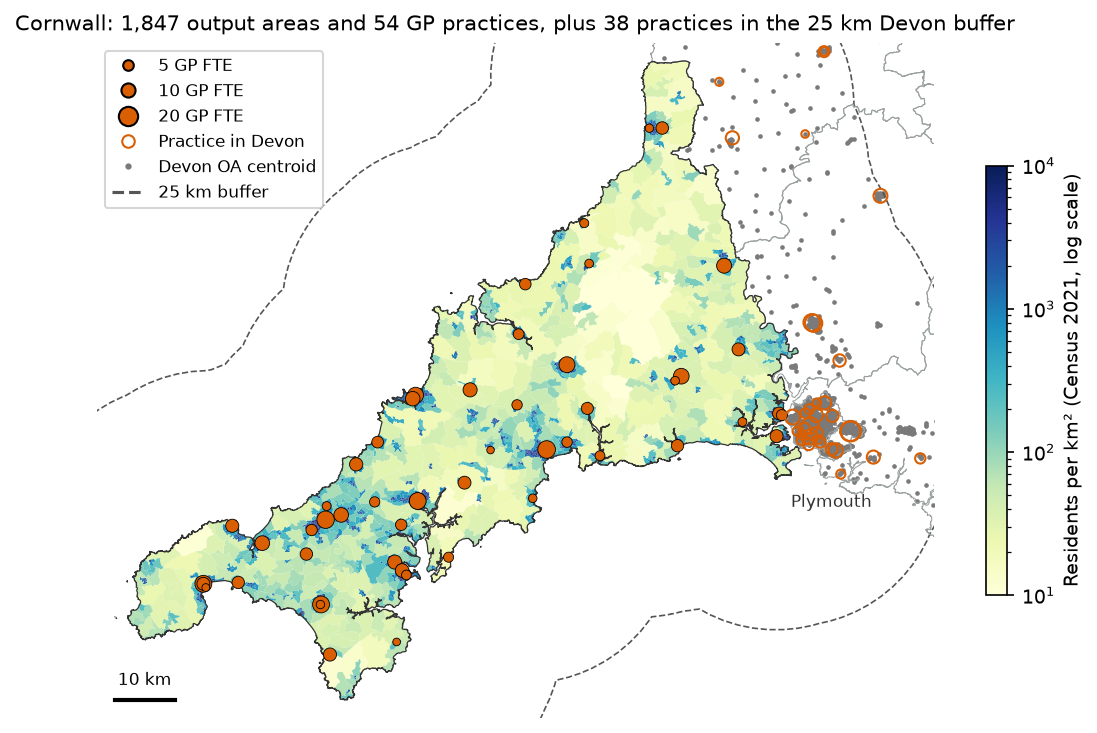
Access in Cornwall depends on GPs and patients in Plymouth and west Devon as well, so the script takes supply and demand from a 25 km buffer around Cornwall and reports access only for Cornwall. The Isles of Scilly have no road link and are left out.
lads = arcgis(LAD_URL, DATA / "lads.geojson", **envelope(130000, 0, 300000, 140000))cornwall = lads[lads.LAD26CD == LAD].geometry.iloc[0]study = cornwall.buffer(BUFFER_M)                                  # 25 km
pop = read_zip_csv(download(TS001, DATA / "census2021-ts001.zip"), "-oa.csv")pop = pop.rename(columns={"geography code": "OA21CD", "Residence type: Total; measures: Value": "pop"})pwc = arcgis(OA_PWC_URL, DATA / "oa_pwc.geojson", **envelope(*study.bounds))pwc = pwc[pwc.within(study)].merge(pop[["OA21CD", "pop"]], on="OA21CD").reset_index(drop=True)oas = arcgis(OA_URL, DATA / "cornwall_oas.geojson", where="LSOA21NM LIKE 'Cornwall %'")pwc["in_cornwall"] = pwc.OA21CD.isin(oas.OA21CD)
arcgis() is a 15-line helper that pages through an ONS ArcGIS FeatureServer layer (2,000 features per request) and caches the result as GeoJSON. For supply, the script joins the practice list to the workforce file on the practice code, geocodes the 142 TR, PL and EX postcodes with one bulk request per 100 postcodes to postcodes.io, and keeps the practices inside the buffer:
prac = pmap[pmap.PRACTICE_POSTCODE.str.match(r"^(TR|PL|EX)\d")][ ["PRACTICE_CODE", "PRACTICE_NAME", "PRACTICE_POSTCODE", "ICB_NAME"]].copy()prac = prac.merge(plist[["CODE", "NUMBER_OF_PATIENTS"]].rename(columns={"CODE": "PRACTICE_CODE"}), how="left")gpw["TOTAL_GP_FTE"] = pd.to_numeric(gpw.TOTAL_GP_FTE, errors="coerce")prac = prac.merge(gpw[["PRAC_CODE", "TOTAL_GP_FTE"]].rename(columns={"PRAC_CODE": "PRACTICE_CODE"}), how="left")Cornwall: 3,549 km2 | with a 25 km buffer: 14,979 km2 (much of it sea)3,183 output areas in the buffered study area, 980,749 residents (Census 2021) in Cornwall: 1,847 OAs, 570,334 residents; in the buffer (Devon): 1,336 OAs, 410,415 residentsEngland: 6,124 practices in the October 2026 list; 6,143 in the August 2026 workforce file142 practices with TR, PL or EX postcodes; 0 postcodes not found92 practices in the buffered study area: 54 in Cornwall, 38 in Devonpractices with no GP FTE in the workforce file: 0Cornwall: 600,920 registered patients, 409.0 GP FTE (0.681 per 1,000 registered patients); 1,493 patients per GP FTE across the study areaCornwall practice size: median 9,070 patients, median 7.3 GP FTETwo numbers are worth noticing. Cornwall’s practices have 600,920 registered patients but only 570,334 residents at the 2021 Census: list sizes include people who have moved away or died and not yet been removed, second-home owners and students. That is one more reason to use Census residents for demand. And “Devon” here means Devon and Plymouth: 38 practices in the buffer, most of them in Plymouth.
Step 2: a drive-time network with OSMnx
OSMnx usually downloads roads from the Overpass API. On the day this was written every public Overpass server I tried returned errors or timed out, and the main server’s usage policy asks scripted users to keep queries small. So the script builds the same graph from Geofabrik’s Cornwall and Devon extracts instead. It uses pyosmium to keep the ways that OSMnx’s network_type="drive" filter would keep and touch the buffered study area, writes them to an .osm file and reads that with ox.graph_from_xml. This takes about two minutes on the first run and is cached as GraphML.
G = ox.graph_from_xml(osm_file, simplify=True)G = ox.routing.add_edge_speeds(G) # km/h from maxspeed, else the mean for that road typeG = ox.routing.add_edge_travel_times(G) # secondsG = ox.truncate.largest_component(G, strongly=True)G = ox.project_graph(G, to_crs="EPSG:27700")Keeping only the largest strongly connected component matters for drive times: it removes one-way fragments and private estates from which you cannot get back to the main network, so every pair of nodes has a finite travel time.
Snapping and the travel-time matrix
Each output-area centroid and practice is snapped to its nearest graph node. The straight-line hop to that node is added at 20 km/h at both ends of the trip, so a centroid 500 m from the nearest road is not treated as being on it. One Dijkstra search per practice on the reversed graph gives the drive time from every node to that practice, so the 3,180 × 92 matrix needs only 92 searches. If you are new to OSMnx routing, see street network analysis with OSMnx.
edges = pd.DataFrame([(pos[a], pos[b], d["travel_time"]) for a, b, d in G.edges(data=True)], columns=["u", "v", "t"])edges = edges.groupby(["u", "v"], as_index=False).t.min()   # keep the fastest of any parallel edgesW = csr_matrix((edges.t, (edges.u, edges.v)), shape=(len(nodes), len(nodes)))
def snap(points):    """Nearest graph node for each point, the hop to it in minutes and its length in metres."""    ids, dist = ox.distance.nearest_nodes(G, points.geometry.x, points.geometry.y, return_dist=True)    dist = np.asarray(dist)    return np.array([pos[i] for i in ids]), dist / 1000 / SNAP_KMH * 60, dist
d_node, d_hop, d_dist = snap(pwc)s_node, s_hop, s_dist = snap(prac)to_prac = dijkstra(W.T.tocsr(), directed=True, indices=s_node) / 60 # practices x nodes, minutesT = to_prac[:, d_node].T + d_hop[:, None] + s_hop[None, :] # OAs x practices, minutes46,322 nodes, 105,181 edges (largest strongly connected component); 7 sedge speeds: median 40 km/h; 4.0% of edges at 96 km/h or moredropping 3 OA(s) more than 2 km from the network: E00102210, E00102212, E00102175 (781 residents, in Cornwall: 0)snap distance: OA centroids median 40 m, 95th percentile 241 m, max 1903 m; practices median 49 m, max 200 mtravel-time matrix: 3,180 OAs x 92 practices in 0.4 s; unreachable pairs: 0The three dropped output areas are in Devon, more than 2 km from any drivable road in the extract, and none is in Cornwall. Check the snap distances whenever you do this: a long snap usually means a missing road, an island or a centroid in the wrong place.
Step 3: the baseline, drive time to the nearest practice
The simplest access measure is the travel time to the nearest facility. It is easy to explain and it is what most people mean by “access”.
pwc["nearest_min"] = T.min(axis=1)pwc["nearest_code"] = prac.PRACTICE_CODE.to_numpy()[T.argmin(axis=1)]Cornwall residents' drive time to the nearest GP practice: mean 3.8 min, median 3.0 min, max 14.7 min more than 10 min: 15,215 residents (2.7%) more than 15 min: 0 residents (0.0%) more than 20 min: 0 residents (0.0%)Cornwall OAs whose nearest practice is in Devon: 12 (3,398 residents)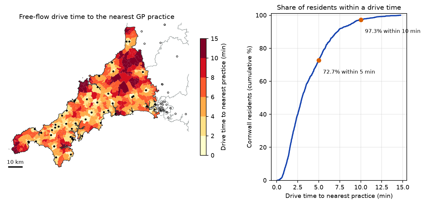
On this measure Cornwall looks well served: nobody is more than 15 minutes from a surgery. But the measure ignores capacity entirely, and 12 Cornish output areas near the Tamar have their nearest practice in Devon. Floating catchment methods address both.
Step 4: 2SFCA and E2SFCA with the access package
The 2SFCA method has two steps, both within a travel-time catchment d₀:
- For each practice j, divide its supply Sj (GP FTE) by the population of every output area k within d₀ of it: Rj = Sj / Σk: tkj ≤ d₀ Pk.
- For each output area i, add up the ratios of every practice within d₀: Ai = Σj: tij ≤ d₀ Rj.
The result is in GP FTE per resident; multiplying by 1,000 gives GP FTE per 1,000 residents. Because each practice’s ratio is shared out among everyone who can reach it, the population-weighted average of Ai over the whole area stays close to the overall supply-to-population ratio, apart from edge effects.
E2SFCA puts a weight W on both sums, so people and practices further away count less: here the step weights from Luo and Qi (2009), 1 for 0–10 minutes, 0.68 for 10–20 and 0.22 for 20–30. The script also runs a continuous Gaussian decay (σ = 15 minutes) for comparison.
The access package wants three tables in long format: demand, supply and a cost table with one row per origin-destination pair. Pairs over 60 minutes are dropped to keep the table small.
cost = (pd.DataFrame(T, index=pwc.OA21CD, columns=prac.PRACTICE_CODE).stack().rename("minutes") .rename_axis(["origin", "dest"]).reset_index())cost = cost[cost.minutes <= 60]STEP = {10: 1.0, 20: 0.68, 30: 0.22} # Luo and Qi (2009) zone weightsSIGMA = 15 # Gaussian decay: weight 0.61 at 15 min, 0.14 at 30 minA = Access(demand_df=pwc[["OA21CD", "pop"]], demand_index="OA21CD", demand_value="pop", supply_df=prac[["PRACTICE_CODE", "TOTAL_GP_FTE"]], supply_index="PRACTICE_CODE", supply_value="TOTAL_GP_FTE", cost_df=cost, cost_origin="origin", cost_dest="dest", cost_name="minutes")A.two_stage_fca(name="2sfca", max_cost=30)A.enhanced_two_stage_fca(name="e2sfca", max_cost=30, weight_fn=weights.step_fn(STEP))A.enhanced_two_stage_fca(name="g2sfca", max_cost=60, weight_fn=weights.gaussian(SIGMA))acc = A.access_df.reindex(pwc.OA21CD).fillna(0) * 1000 # GP FTE per 1,000 residentsfor name in ("2sfca", "e2sfca", "g2sfca"): pwc[name] = acc[f"{name}_TOTAL_GP_FTE"].to_numpy()access_df names the result columns <name>_<supply column>. It also contains the demand column, so select the columns you want rather than joining the whole frame back onto your data.
The same thing in ten lines of NumPy
The method is simple enough to write as two matrix products, which is a good check and makes the sensitivity tests below fast:
def fca(T, demand, supply, weight):    """Vectorised 2SFCA: weight is a function of the travel-time matrix (OAs x practices)."""    Wt = weight(T)    ratio = supply / (Wt.T @ demand)          # step 1: supply-to-demand ratio for each practice    return Wt @ ratio * 1000                  # step 2: sum the ratios each OA can reach
binary = lambda t, d=30: (t <= d).astype(float)step = lambda t: np.select([t <= 10, t <= 20, t <= 30], [1.0, 0.68, 0.22], 0.0)gauss = lambda t: np.where(t <= 60, np.exp(-t ** 2 / (2 * SIGMA ** 2)), 0.0)cost table: 189,308 OA-practice pairs within 60 min2sfca: numpy vs access max abs difference 2.22e-16e2sfca: numpy vs access max abs difference 6.66e-16g2sfca: numpy vs access max abs difference 4.44e-16Cornwall overall: 0.717 GP FTE per 1,000 residents (Cornwall practices / Cornwall residents)2sfca mean 0.721 | median 0.749 | OA 10th-90th pct 0.442-0.935 | min 0.228 max 1.111 | CV 0.27e2sfca mean 0.702 | median 0.692 | OA 10th-90th pct 0.434-0.942 | min 0.178 max 1.116 | CV 0.29g2sfca mean 0.704 | median 0.696 | OA 10th-90th pct 0.447-0.932 | min 0.215 max 1.060 | CV 0.25Spearman rank correlation, nearest-practice time vs E2SFCA (Cornwall OAs): -0.22The package and the NumPy version agree to rounding error. The population-weighted means (0.70–0.72) are close to the county ratio of 0.717, as they should be; the small differences come from people in Cornwall using Plymouth practices and the other way round.
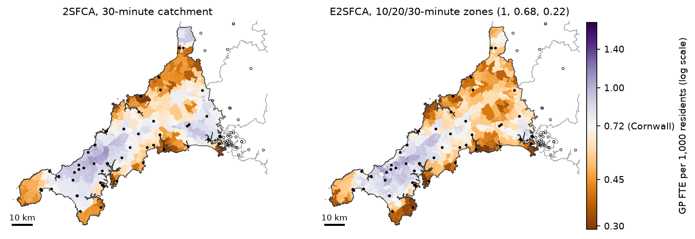
The binary 2SFCA gives broad, smooth zones, because everyone within 30 minutes counts equally. E2SFCA gives more weight to the nearest practices and sharpens the pattern. Reverse-geocoding the lowest-scoring 10% of output areas to electoral wards with postcodes.io puts the most residents in Torpoint, Looe West, Padstow, Rame Peninsula and St Germans, Mullion and St Keverne (the Lizard), and St Goran, Tregony and the Roseland. The highest scores are in Camborne, Redruth, Pool and Truro, where many practices sit close together.
Step 5: choosing the catchment threshold and the decay function
Both the threshold d₀ and the shape of the decay are choices, and they change the answer. The script reruns 2SFCA with six thresholds:
for d in [10, 15, 20, 30, 45, 60]: x = fca(T, pop_all, fte, lambda t, d=d: binary(t, d))[inC] rho = pd.Series(x).corr(pd.Series(base30), method="spearman")10 min: OA 10th-90th pct 0.380-1.101 | CV 0.44 | residents with no practice in reach 15,215 | Spearman vs 30 min 0.1915 min: OA 10th-90th pct 0.447-1.065 | CV 0.32 | residents with no practice in reach 0 | Spearman vs 30 min 0.5420 min: OA 10th-90th pct 0.409-1.012 | CV 0.34 | residents with no practice in reach 0 | Spearman vs 30 min 0.7730 min: OA 10th-90th pct 0.442-0.935 | CV 0.27 | residents with no practice in reach 0 | Spearman vs 30 min 1.0045 min: OA 10th-90th pct 0.616-0.966 | CV 0.18 | residents with no practice in reach 0 | Spearman vs 30 min 0.3260 min: OA 10th-90th pct 0.561-1.037 | CV 0.25 | residents with no practice in reach 0 | Spearman vs 30 min -0.11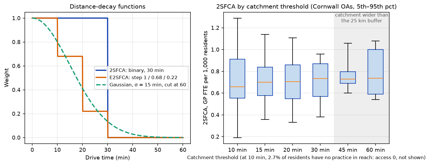
Three lessons:
- Too short a catchment fragments the map. At 10 minutes, 15,215 people (2.7%) have no practice in reach and score zero, and practices’ ratios depend on tiny, arbitrary catchments. The coefficient of variation (CV) jumps to 0.44.
- Moderate changes keep the ranking. 20 and 30 minutes give similar rankings (Spearman 0.77), so the conclusions about which areas are worst are fairly stable in that range.
- Long catchments smooth everything out, and here they also hit the edge of the data. At 45 and 60 minutes, almost everyone can reach almost every practice, so the scores converge. But a 45-minute catchment from east Cornwall reaches well beyond the 25 km buffer, where we have no supply or demand, so those results are biased. If you need long catchments, widen the buffer as well.
A threshold of 30 minutes is a common choice for primary care in rural areas in the literature, and it is a reasonable upper bound on how far people in Cornwall drive to their own practice. In a city, 10–15 minutes, or walking and public transport times, would be more sensible. The decay function matters less than the threshold here: the step-function E2SFCA and the Gaussian version have similar means (0.702 and 0.704) and spreads (CV 0.29 and 0.25). The Gaussian is smoother and avoids the cliff-edges of the step weights; the step weights are easier to explain to a non-technical audience.
Step 6: edge effects at the Devon border
Floating catchments cross boundaries. People in Saltash and Torpoint can use practices in Plymouth, and Plymouth’s residents compete for the same practices. To see how much this matters, the script computes E2SFCA three ways:
variants = { "Cornwall only": fca(T[inC][:, pC], popC.astype(float), fte[pC], step), "+ Devon practices only": fca(T[inC], popC.astype(float), fte, step), "+ Devon practices and residents": pwc.loc[inC, "e2sfca"].to_numpy(),}population-weighted mean E2SFCA (GP FTE per 1,000) by distance from the Devon border (km): Cornwall only + Devon practices only + Devon practices and residents residentsband0-5 0.568 3.750 0.640 48791.05-10 0.549 3.211 0.549 33329.010-20 0.681 1.782 0.512 39396.020-40 0.655 0.673 0.596 81850.040+ 0.770 0.770 0.768 366968.0Cornwall only: vs full buffer, OAs within 10 km of the border: median -7.7%, range -48.0% to +79.6%; beyond 40 km max |diff| 3.7%+ Devon practices only: vs full buffer, OAs within 10 km of the border: median +413.3%, range +55.4% to +2384.0%; beyond 40 km max |diff| 3.7%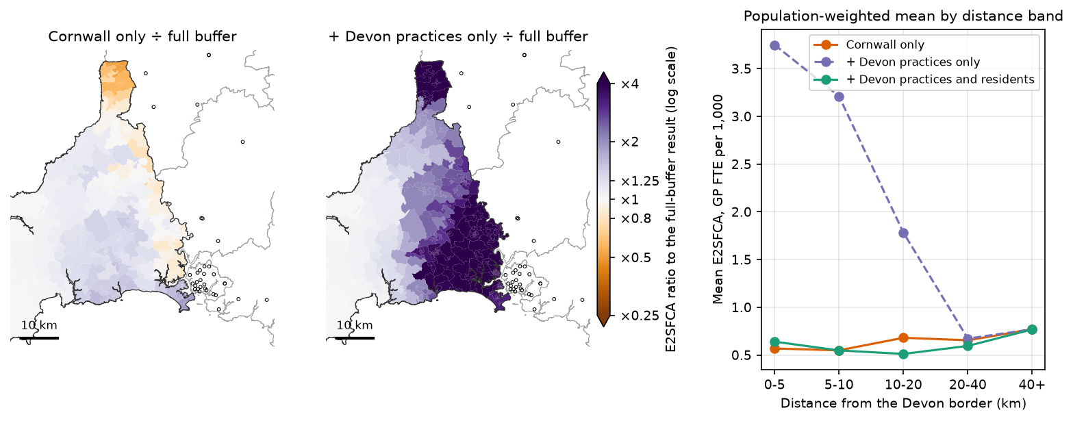
- Ignoring the buffer completely (“Cornwall only”) changes scores within 10 km of the border by −48% to +80% (median −7.7%). Near the Tamar it understates access, because Plymouth’s practices are missing. 10–20 km in, it overstates access, because the Cornish practices near the border no longer have Plymouth residents competing for them.
- Adding outside supply without outside demand is worse. Plymouth’s practices are then shared only among Cornish residents, and scores near the border inflate by 55% to 2,384%. This is the most common mistake in published 2SFCA studies: if you include facilities beyond the boundary, include the people who use them as well.
- Far from the border it does not matter. Beyond 40 km, the three versions differ by at most 3.7%.
The rule is simple: take supply and demand from a buffer at least as wide as your longest catchment, and report results only for the core area.
Step 7: nearness and access disagree
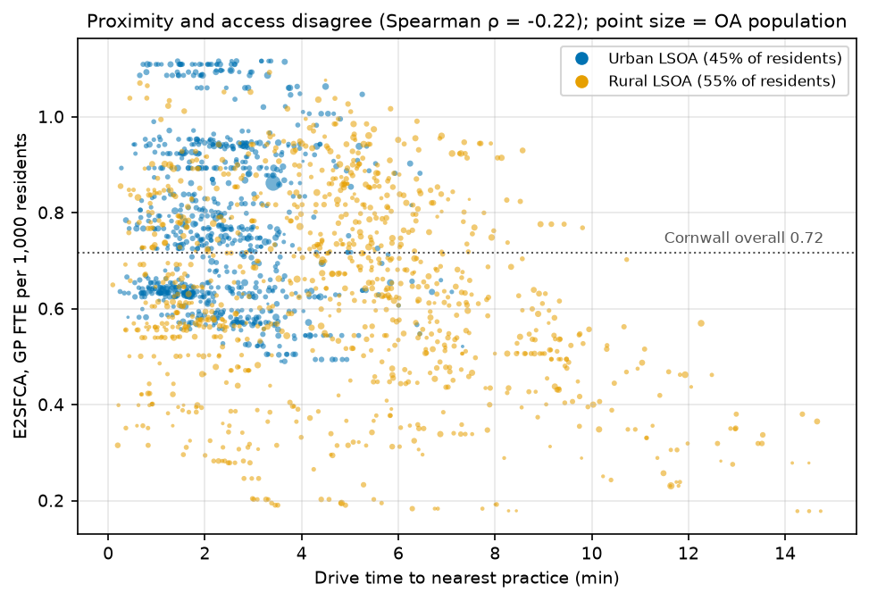
Rural: 311,640 residents (55%) | nearest practice 4.8 min | 2SFCA 0.684 | E2SFCA 0.643 GP FTE per 1,000Urban: 258,694 residents (45%) | nearest practice 2.5 min | 2SFCA 0.766 | E2SFCA 0.773 GP FTE per 1,000lowest-access decile of OAs (E2SFCA < 0.434): 49,119 residents, 0% urban, mean nearest-practice time 6.1 minThe two measures answer different questions. Nearest-practice time says how far people must travel. E2SFCA says how much GP capacity is available for them once everyone else who can reach the same practices is counted. Their rank correlation is only −0.22. Some urban areas a minute from a practice score below 0.6 because that practice serves a large town; some rural areas eight minutes away score above average because their practice has few competitors. Every one of the lowest-access 10% of output areas is rural, though: rural Cornwall is both further from GPs and has fewer GPs per head within reach.
Limitations and honest caveats
- Potential access, not use. 2SFCA measures the supply people could reach, assuming they choose among all practices in the catchment. In England patients register with one practice, practice boundaries restrict who can register, and many people choose a practice near work rather than home.
- Supply is GP FTE only. Nurses, clinical pharmacists, paramedics and physician associates now provide a large share of appointments. The workforce file has their FTE too, if you want a broader measure of capacity. The workforce data (August 2026) and practice list (October 2026) are two months apart.
- Main surgeries only, at postcode centroids. Branch surgeries are not in the open practice lists, so access in villages with a branch surgery is understated. Postcode centroids are close to the building in towns but can be some way off in the countryside. A branch surgery or a missing ferry shows up as poor access, so check the lowest-scoring areas against local knowledge before acting on them.
- Free-flow car travel times. OSMnx assigns speed limits, or typical speeds where there is no limit, so these are free-flow times with no congestion, parking or junction delays. Real times are longer, especially in summer in Cornwall, and households without a car depend on bus times instead. The Torpoint ferry is not in the drive network, because OSM ferry routes are not highways, so Torpoint’s access to Plymouth is understated: it is one of the lowest-scoring wards.
- Population is where people sleep. Census residents at output-area centroids leave out the large summer tourist population and second-home owners, which add real demand in coastal Cornwall.
- Scale and zoning (MAUP). Results depend on the areal unit. Output areas are about as fine as open population data goes; LSOAs would smooth the pattern.
- The Isles of Scilly have their own practice and no road link, so they are excluded.
Frequently asked questions
What is the two-step floating catchment area method?
2SFCA is a way to measure spatial access to a service that accounts for both distance and capacity. In step 1, each facility’s capacity is divided by the population within a travel-time catchment around it. In step 2, each neighbourhood’s score is the sum of the ratios of all the facilities within the same catchment of it. The result is capacity per head, such as GP FTE per 1,000 residents, that each place can reach. Luo and Wang introduced it in 2003, building on Radke and Mu (2000).
What is the difference between 2SFCA and E2SFCA?
2SFCA treats everyone and every facility inside the catchment equally and ignores everything outside it. E2SFCA, the enhanced version by Luo and Qi (2009), applies a distance-decay weight in both steps, usually a step function over travel-time zones, so nearer people and facilities count more. Other variants use a continuous Gaussian or kernel decay (KD2SFCA), add competition between facilities (3SFCA), or vary the catchment size by place.
How do I calculate 2SFCA in Python?
Use the PySAL access package: build a demand table, a supply table and a long cost table of origin-destination travel times, create an Access object and call two_stage_fca(max_cost=...) or enhanced_two_stage_fca(max_cost=..., weight_fn=weights.step_fn({...})). Alternatively, with a dense travel-time matrix T, compute W = weight(T), then ratio = supply / (W.T @ demand) and access = W @ ratio, as in the NumPy version above.
What catchment size should I use for 2SFCA?
There is no universal value. Use the time people realistically travel for that service: often 30 minutes by car for GPs in rural areas, and 10–15 minutes in cities or for walking. Report the threshold you chose and test a range of values, as in Step 5. Make sure the buffer of data around your study area is at least as wide as the catchment.
How do I get road network travel times for accessibility analysis in Python?
Build a drivable network with OSMnx, add speeds and travel times with ox.routing.add_edge_speeds and ox.routing.add_edge_travel_times, snap your origins and destinations with ox.distance.nearest_nodes, and run a shortest-path search. For whole matrices, convert the graph to a SciPy sparse matrix and use scipy.sparse.csgraph.dijkstra, which is much faster than looping in NetworkX. For public transport or congested times, use a routing engine such as r5py or OSRM instead.
Is 2SFCA better than the distance to the nearest GP?
They measure different things, and it is worth reporting both. The nearest-facility time is easy to communicate and matters for urgent travel. 2SFCA captures crowding: a practice nearby may be stretched across a large population. In Cornwall the two have a rank correlation of only −0.22, so they would pick out different areas as under-served.
Next steps
- Part 2: decide where new services should go, using the same network and travel times, in location-allocation in Python with spopt. It solves p-median, p-center and maximal covering problems for new urgent-care sites in Cornwall.
- Learn the basics of drive and walk networks, routes and isochrones in street network analysis with OSMnx.
- Test whether low-access areas cluster with hot spot analysis in Python. The script writes
data/oa_access.csvwith every score. - Attach the scores to other area data with spatial joins in GeoPandas, or aggregate them to a regular grid with H3 hexagon grids in Python.
Data and licences
- GP practices and workforce: NHS England, Patients Registered at a GP Practice, October 2026 and General Practice Workforce, 31 August 2026, from digital.nhs.uk. Contains public sector information licensed under the Open Government Licence v3.0.
- Postcode locations: postcodes.io, based on the ONS Postcode Directory. Contains OS data © Crown copyright and database right 2026; contains Royal Mail data © Royal Mail copyright and database right 2026; source: Office for National Statistics licensed under the Open Government Licence v3.0.
- Population: ONS, Census 2021 TS001: number of usual residents in households and communal establishments, from Nomis. Open Government Licence v3.0.
- Boundaries and centroids: ONS, Output Areas (December 2021) Population Weighted Centroids (V4), Output Areas (2021) Boundaries EW BGC (V2), LSOA (2021) Boundaries with Rural Urban Classification and Local Authority Districts (May 2026) Boundaries UK BGC, from the Open Geography Portal. Source: Office for National Statistics licensed under the Open Government Licence v3.0. Contains OS data © Crown copyright and database right 2026.
- Roads: © OpenStreetMap contributors, available under the Open Database Licence. Cornwall and Devon extracts from Geofabrik, downloaded on 27 October 2026.
- Further reading: Luo, W. and Wang, F. (2003), “Measures of spatial accessibility to health care in a GIS environment”, Environment and Planning B 30: 865–884; Luo, W. and Qi, Y. (2009), “An enhanced two-step floating catchment area (E2SFCA) method for measuring spatial accessibility to primary care physicians”, Health & Place 15: 1100–1107; Saxon, J. et al. (2022), “An open software environment to make spatial access metrics more accessible”, Journal of Computational Social Science 5: 265–284.
- Code:
gp_access_2sfca.py, tested with Python 3.12.0, access 1.1.10.post3, osmnx 2.1.1, networkx 3.7, osmium 4.3.2, geopandas 1.2.0, pyogrio 0.13.0, shapely 2.2.0, pyproj 3.8.0, numpy 2.5.4, pandas 3.1.0, scipy 1.18.1, pyarrow 26.0.0, matplotlib 3.11.2 and requests 2.34.2.
Key terms
- Spatial accessibility
- How easily people in a place can reach a service, taking account of both the travel cost and how much service there is for how many people.
- 2SFCA
- The two-step floating catchment area method (Luo and Wang, 2003). Step 1 computes a supply-to-demand ratio for each facility within a travel-time catchment. Step 2 sums the ratios of all facilities each demand location can reach within the same catchment.
- E2SFCA
- Enhanced 2SFCA (Luo and Qi, 2009). It weights the population and the ratios by travel-time zones, so nearer people and nearer practices count more, instead of treating everything within the catchment equally.
- Distance decay
- The fall in the chance or willingness to use a service as the travel cost rises. In floating catchment methods it is a weight function of travel time, such as a step function or a Gaussian curve.
- Population-weighted centroid
- A point for an area that sits where its residents live rather than at its geometric centre. The ONS publishes them for 2021 output areas and LSOAs.
- GP FTE
- Full-time equivalent GPs: the number of GPs scaled by their contracted hours, where 37.5 hours a week is 1 FTE. NHS England publishes it by practice in the General Practice Workforce statistics.
- Edge effect
- Bias near the edge of a study area because the services and people just outside it are left out of the calculation.
Data for this tutorial
- Nomis · Census 2021 table TS001 (usual residents) by output area
- Open Geography Portal · ONS 2021 output area boundaries and population-weighted centroids, LSOA rural-urban classification and local authority boundaries
- Geofabrik OpenStreetMap extract (England) · Cornwall and Devon .osm.pbf extracts used to build the drive network
- Patients Registered at a GP Practice (NHS England Digital) · October 2026 practice codes and postcodes, used to locate the GP practices
- General Practice Workforce (NHS England Digital) · Full-time equivalent GPs per practice, 31 August 2026, used as the supply
- postcodes.io · Free bulk postcode geocoding for the practice postcodes
Licences and formats for each source are listed in the GIS data sources catalogue.