Location-allocation in Python: p-median, p-center and maximal covering (MCLP) with spopt
Solve location-allocation problems in Python with spopt and the CBC solver: the p-median, p-center and maximal covering location problem (MCLP). Choose sites for new urgent-care or mobile clinic bases among Cornwall's community buildings, on OSMnx drive times and Census 2021 population, compare the three answers on maps and charts, draw the trade-off curve as the number of sites grows, and see how problem size drives solve time.
- Level
- Intermediate
- Tested with
- Python 3.12
- Source code
- Download scripts
Key takeaways
- Location-allocation chooses p sites from a list of candidates to optimise an objective over a travel-cost matrix. spopt builds the three classic models from a NumPy matrix in one line each, PMedian, PCenter and MCLP, and solves them with any PuLP solver, including the CBC solver that ships with PuLP.
- The three objectives give three different answers. For six new sites among 144 Cornish community buildings, p-median gives the lowest mean drive time (10.6 minutes), p-center the lowest worst case (22.1 minutes) and MCLP the most residents within 15 minutes (85.9%). Not one site is chosen by all three.
- Each model is good at its own objective and can be poor at the others. The MCLP solution leaves its worst-served area 42.8 minutes away; the p-center solution reaches only 69% of residents within 15 minutes.
- Returns diminish quickly. Going from one site to two saves 7.8 minutes on the average trip; going from 11 to 12 saves 0.5. The trade-off curve, not a single optimum, is the most useful output for a planning discussion.
- Problem size matters more than the model. p-median on 336 LSOAs has 49k variables and solves in about 3 seconds; on 1,847 output areas it has 266k variables and takes over 3 minutes, for the same answer. The direct p-center model took over two minutes, but solving it as a sequence of set-covering problems gives the same optimum in about 4 seconds.
Before you start
- Part 1 of this series, or at least its drive network: the script reuses Part 1's cached graph if it finds it
- Python 3.10+ with spopt, pulp, osmnx, osmium, geopandas, scipy, matplotlib and requests (PuLP ships with the CBC solver)
- An internet connection if Part 1 has not been run: the script then downloads about 90 MB of open data and builds the graph itself, which takes about 5 minutes
Short answer: to solve a location-allocation problem in Python, build a matrix of travel times from demand points (rows) to candidate sites (columns), then let spopt build the model and PuLP’s bundled CBC solver solve it:
import pulpfrom spopt.locate import PMedian, PCenter, MCLP
solver = pulp.PULP_CBC_CMD(msg=False)pmed = PMedian.from_cost_matrix(T, population, p_facilities=6).solve(solver)            # least total timepcen = PCenter.from_cost_matrix(T, p_facilities=6).solve(solver)                        # least worst timemclp = MCLP.from_cost_matrix(T, population, service_radius=15, p_facilities=6).solve(solver)  # most covered
For six new urgent-care or mobile clinic bases among 144 community buildings in Cornwall, the p-median solution gives a mean drive of 10.6 minutes, the p-center solution a worst case of 22.1 minutes, and the maximal covering (MCLP) solution puts 85.9% of residents within 15 minutes. The three solutions share no sites, so the choice of objective is a policy decision, not a technical one.
Part 1 of this series measured how good access to GP practices in Cornwall is now, with the two-step floating catchment area method. This part asks the planning question that follows: if you could open a handful of new sites, where should they go? That is a facility location problem. The classic models each formalise a different idea of “best”: the lowest average journey, the fairest worst journey, or the most people within a standard.
You will learn how to:
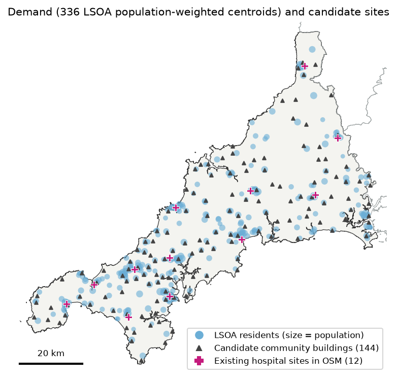
- set up demand (Census 2021 residents at LSOA population-weighted centroids) and candidate sites (community buildings and town halls from OpenStreetMap);
- reuse Part 1’s OSMnx drive network to build a 336 × 156 travel-time matrix in under two seconds;
- solve the p-median, p-center and MCLP models with spopt and CBC, and compare their answers on maps and charts;
- draw the trade-off curve as the number of sites p goes from 1 to 12;
- measure solve time against problem size, and speed up the p-center model by solving it as a series of set-covering problems;
- add new sites to an existing network of 12 NHS hospital sites with fixed facilities.
What you need from Part 1
This tutorial uses the same study area (Cornwall, without the Isles of Scilly) and the same road network as Part 1. The script looks in Part 1’s data/ folder (../spatial-accessibility-2sfca-python/data/) for:
cornwall_drive.graphml, the drive network for Cornwall plus a 25 km buffer, with free-flow travel times on every edge;cornwall-latest.osm.pbf, the Geofabrik extract, which is also the source of the candidate sites;- the cached ONS boundaries, output-area centroids and Census table.
If Part 1 has not been run, you do not need to run it. location_allocation.py contains the same downloaders and graph builder, and it builds everything in its own data/ folder. Either way, one command reproduces every number and figure in this post:
pip install -r requirements.txtpython location_allocation.pyWith Part 1’s cache, the whole script takes about 10 minutes, almost all of it in the two deliberately slow benchmarks in Step 5.
The question and the data
The question: NHS Cornwall wants to open six new bases for urgent treatment, or for mobile clinics that visit from a base, in buildings it can rent: village halls, community centres and town halls. Which six minimise travel for residents? And what if they are added to the existing hospital sites instead of replacing them?
The question is illustrative. The real decision would also weigh staffing, opening hours, the existing urgent treatment centres, and the buildings’ size and condition.
| Role | Dataset | Source |
|---|---|---|
| Demand | Usual residents by 2021 LSOA and output area (TS001) | ONS Census 2021 via Nomis |
| Demand (locations) | LSOA and output area population-weighted centroids (2021) | ONS Open Geography Portal |
| Candidate sites | amenity=community_centre, village_hall and townhall |
OpenStreetMap via Geofabrik |
| Existing sites | amenity=hospital named “… Hospital” |
OpenStreetMap via Geofabrik |
| Travel cost | Free-flow drive times on the Part 1 network | OpenStreetMap via OSMnx |
Why LSOAs, when Part 1 used output areas? Location models grow with the number of demand points times the number of candidates. Cornwall’s 336 LSOAs (median 1,611 residents) keep the p-median model to about 49,000 variables. Step 5 repeats the analysis on 1,847 output areas to show what that costs and whether it changes the answer.
Step 1: demand and candidate sites
The LSOA population-weighted centroids come from the ONS Open Geography Portal, and the populations from the Census 2021 TS001 table. Only LSOAs whose output areas are in Cornwall are kept:
lsoa = arcgis(LSOA_PWC_URL, DATA / "cornwall_lsoa_pwc.geojson", **envelope(*cornwall.bounds))lsoa = lsoa[lsoa.LSOA21CD.isin(oas.LSOA21CD)]lsoa = lsoa.merge(read_zip_csv(ts001, "-lsoa.csv").rename(columns=col)[["code", "pop"]], left_on="LSOA21CD", right_on="code").drop(columns="code").reset_index(drop=True)The candidates come from the Geofabrik extract that Part 1 downloaded. osm_places() reads it once with pyosmium, keeping nodes and building outlines tagged as community centres, village halls, town halls or hospitals, and caches them as a GeoPackage. Many villages have two or three halls within a few hundred metres, which add nothing to the model but variables, so thin() keeps at most one candidate per 2 km, preferring named ones:
def thin(gdf, min_dist):    """Greedy thinning: keep a point only if it is at least min_dist from every point already kept."""    gdf = gdf.assign(named=gdf.name.fillna("").ne("")).sort_values(["named", "osm"], ascending=[False, True])    kept, xy = [], gdf.get_coordinates().to_numpy()    for i in range(len(gdf)):        if not kept or np.min(np.hypot(*(xy[kept] - xy[i]).T)) >= min_dist:            kept.append(i)    return gdf.iloc[kept].drop(columns="named").reset_index(drop=True)
hosp = places[(places.kind == "hospital") & places.name.str.endswith("Hospital") & (places.name != "The Duchy Hospital")]cand = thin(places[places.kind == "candidate"], THIN_M)336 Cornwall LSOAs, 570,320 residents (Census 2021), median 1,611 per LSOAfor the problem-size benchmark: 1,847 Cornwall OAs, 570,334 residentsOSM features in Cornwall: {('candidate', 'community_centre'): 205, ('candidate', 'townhall'): 22, ('hospital', 'hospital'): 18}NHS hospital sites kept: Bodmin Hospital, Camborne Redruth Community Hospital, Falmouth Hospital, Helston Community Hospital, Launceston Community Hospital, Liskeard Community Hospital, Newquay Hospital, Royal Cornwall Hospital, St Austell Community Hospital, St. Michael's Hospital, Stratton Hospital, West Cornwall Hospital144 candidate community buildings after 2 km thinning (from 227); 12 existing hospital sitesCornwall has no amenity=village_hall in OSM: village halls are mapped as community centres. The amenity=hospital tag also picks up a surgery, military medical centres and a historic site, so the script keeps names ending in “Hospital” and drops the one private hospital. That leaves the Royal Cornwall Hospital in Truro and 11 community hospitals. (The LSOA and output-area totals differ by 14 residents because the ONS applies statistical disclosure control to each table separately.)
Step 2: the travel-time matrix
The travel-time code is Part 1’s, applied to new points. snap() finds the nearest network node to each point with ox.distance.nearest_nodes and charges the straight-line hop to it at 20 km/h, a rough allowance for driveways and minor roads that are not in the network. minutes() runs one SciPy Dijkstra search per site on the reversed graph, so each search gives the times to that site from every node:
WT = csr_matrix((edges.t, (edges.u, edges.v)), shape=(len(nodes), len(nodes))).T.tocsr()
def snap(points):    ids, dist = ox.distance.nearest_nodes(G, points.geometry.x, points.geometry.y, return_dist=True)    return np.array([pos[i] for i in ids]), np.asarray(dist) / 1000 / SNAP_KMH * 60
def minutes(demand, sites):    """Drive time in minutes from every demand point (rows) to every site (columns)."""    d_node, d_hop = snap(demand)    s_node, s_hop = snap(sites)    to_site = dijkstra(WT, directed=True, indices=s_node) / 60    return to_site[:, d_node].T + d_hop[:, None] + s_hop[None, :]
T_all = minutes(lsoa, sites)graph from ../spatial-accessibility-2sfca-python/data/cornwall_drive.graphml: 46,322 nodes, 105,181 edges; 6 sLSOA x site matrix (336, 156) and OA x site matrix (1847, 156) in 1.6 s; unreachable pairs: 0existing 12 hospital sites: mean 7.6 min | worst 26.1 min | 90.7% within 15 minBoth matrices, for 2,183 demand points and 156 sites, take 1.6 seconds. The baseline is useful too: with today’s 12 hospital sites, the average resident is a 7.6-minute free-flow drive from the nearest one, the furthest LSOA is 26.1 minutes away, and 90.7% of residents are within 15 minutes.
evaluate() scores any set of open sites the same way, whichever model chose them, by sending each LSOA to its nearest open site:
def evaluate(open_cols, M=T, wt=w): """Population-weighted mean, worst and coverage, each person using the nearest open site.""" t = M[:, open_cols].min(axis=1) return {"mean_min": np.average(t, weights=wt), "max_min": t.max(), "covered_pct": wt[t <= RADIUS].sum() / wt.sum() * 100}Step 3: p-median, p-center and MCLP with spopt
spopt’s from_cost_matrix constructors take the matrix directly. Under the hood they write an integer linear programme with PuLP, and .solve() passes it to any PuLP solver. CBC, an open-source branch-and-cut solver, is bundled with PuLP, so there is nothing else to install:
CBC = lambda: pulp.PULP_CBC_CMD(msg=False, timeLimit=600)
def solve(kind, p, M=T, wt=w, predefined=None):    """Build and solve one spopt model with CBC; return the open columns and the solve time."""    kw = {} if predefined is None else {"predefined_facilities_arr": predefined}    if kind == "p-median":        m = PMedian.from_cost_matrix(M, wt, p_facilities=p, **kw)    elif kind == "p-center":        m = PCenter.from_cost_matrix(M, p_facilities=p, **kw)    else:        m = MCLP.from_cost_matrix(M, wt, service_radius=RADIUS, p_facilities=p, **kw)    t0 = time.perf_counter()    m = m.solve(CBC())    secs = time.perf_counter() - t0    status = pulp.LpStatus[m.problem.status]    opened = [j for j, clients in enumerate(m.fac2cli) if len(clients)] if kind != "mclp" else \        [j for j in range(M.shape[1]) if m.fac_vars[j].value() > 0.5]    return sorted(opened), secs, status, m.problem.numVariables(), m.problem.numConstraints()
Check that the solver finished: here every model reached a proven optimum well inside the 600-second time limit. If the limit stops CBC first, you get the best solution found so far, and PuLP can still report the status as Optimal; m.problem.sol_status is then 2 (integer feasible) rather than 1 (optimal). The open sites are read from the model’s allocation, fac2cli, or from the facility variables fac_vars.
p-median Optimal in 3.5 s (48,528 variables, 48,721 constraints) | mean 10.6 min | worst 24.1 min | 77.9% within 15 min sites: Ertach Kernow; Liskeard Town Hall; Ponsanooth Hall; Quintrell Downs Village Hall; Bethel Methodist Church Sunday School; Ludgvan Village Hallp-center Optimal in 132.1 s (48,529 variables, 49,057 constraints) | mean 12.1 min | worst 22.1 min | 69.4% within 15 min sites: The Basement Youth Centre; Liskeard Town Hall; St. Erme Village Hall; Jacobstow Parish Hall; St Petroc Community Centre; Ludgvan Village Hallmclp Optimal in 0.3 s (480 variables, 337 constraints) | mean 11.9 min | worst 42.8 min | 85.9% within 15 min sites: Gwennap Parish Hall; Church Rooms; Stoke Climsland Village Hall; Community Centre at Indian Queens Pit; St Pirans Hall; Eliot Hallsites chosen by all three models: 0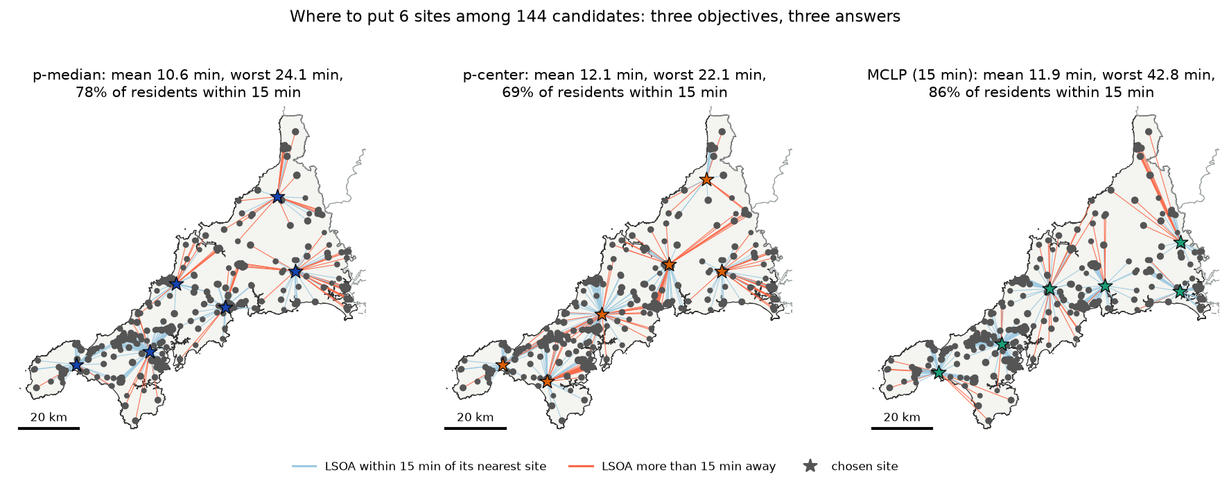
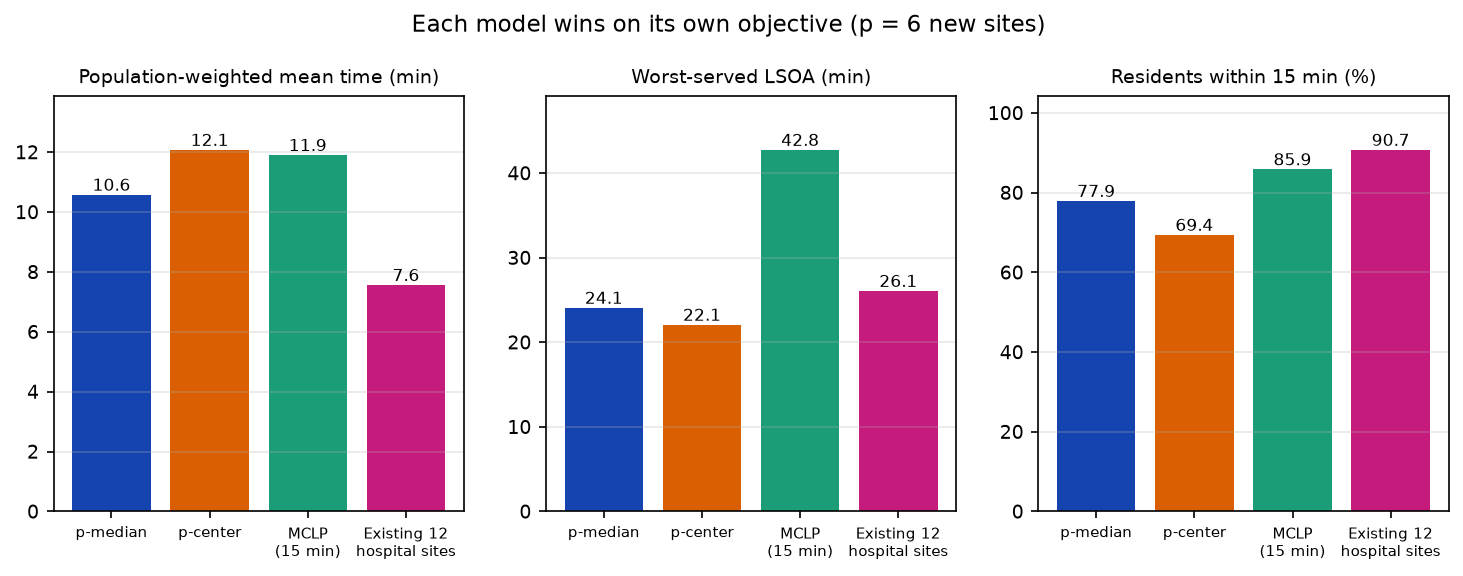
Each model wins on its own objective, as it must, and the differences on the other objectives are large:
- p-median (efficiency) spreads the sites in proportion to population: two in the dense west, one each for St Austell, Newquay and Liskeard, and one in the empty north-east. It has the lowest mean, 10.6 minutes, and a respectable worst case.
- p-center (equity) only cares about the single worst-served LSOA. It pulls sites towards the middle of the county and the far north to bring the worst trip down to 22.1 minutes, at the cost of the mean (12.1) and of coverage (69.4%). Many solutions share the same worst case, so CBC returns one of them, and the others may have quite different means. A common fix is to solve p-center first and then p-median with the worst time as a constraint.
- MCLP (coverage) puts sites where they cover the most people within 15 minutes and ignores everyone beyond it. It covers 85.9% of residents but leaves the far north-east 42.8 minutes from a site, because covering those sparse LSOAs is worth less than covering another town.
Six well-placed sites can almost match the 12 hospitals’ coverage, but not their average: the hospital sites are in the towns, where most people live.
Step 4: the trade-off as p varies
How many sites are worth opening? The script solves all three models for p = 1 to 12 and keeps the results in output/tradeoff.csv:
rows = []for p in P_RANGE: for k in MODELS: if k == "p-center": opened, secs, _ = pcenter_by_covering(T, p) status = "Optimal" else: opened, secs, status, *_ = solve(k, p) rows.append({"model": k, "p": p, "secs": secs, "status": status, **evaluate(opened)})curve = pd.DataFrame(rows) mean_min max_min covered_pctmodel mclp p-center p-median mclp p-center p-median mclp p-center p-medianp1 29.0 27.0 25.3 72.0 51.3 52.2 29.8 14.2 19.02 19.4 19.7 17.5 52.2 39.1 43.0 48.5 33.3 36.83 16.1 17.6 15.0 49.4 35.6 46.5 61.3 34.3 56.94 13.6 15.0 13.3 46.5 26.9 46.5 71.7 44.6 70.85 12.6 12.6 11.8 46.5 25.3 31.0 81.3 67.6 73.26 11.9 12.3 10.6 42.8 22.1 24.1 85.9 68.2 77.97 10.5 12.2 9.7 39.5 21.0 24.4 90.7 65.3 79.28 9.8 11.9 8.9 24.0 19.8 24.4 94.3 72.6 84.99 9.3 9.9 8.4 24.0 17.5 24.4 96.3 90.5 89.510 9.3 10.2 7.8 22.4 16.8 23.7 97.9 93.5 91.811 8.9 9.6 7.3 22.5 15.8 22.6 99.1 97.1 91.812 8.9 9.1 6.9 15.4 15.4 22.6 99.8 99.8 96.1p-median: minutes saved per extra site: 1->2: 7.75, 2->3: 2.52, 3->4: 1.74, 4->5: 1.47, 5->6: 1.22, 6->7: 0.84, 7->8: 0.80, 8->9: 0.55, 9->10: 0.54, 10->11: 0.52, 11->12: 0.45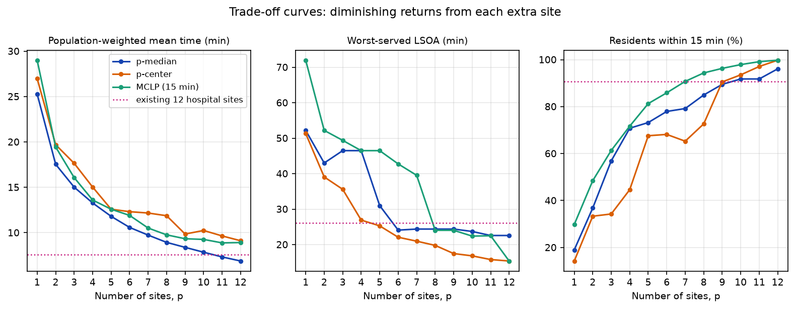
Three things stand out:
- Diminishing returns. The second site saves 7.8 minutes on the average trip; the sixth saves 1.2 and the twelfth 0.5. Where the curve flattens is where extra sites stop being worth much on this measure, which is a more useful thing to show a planning board than a single “optimal” map.
- Curves need not be smooth. Optimal sets are not nested: the best seven sites are not the best six plus one. So a model’s off-objective scores can get worse as p rises, as p-center coverage does from p = 6 to 7, and MCLP’s worst case jumps around.
- The objectives converge as p grows. By p = 12, MCLP and p-center both reach 99.8% coverage and a 15.4-minute worst case. With enough sites, any sensible solution is good; the choice of model matters most when the budget is tight.
Step 5: problem size and solve time
All three models are integer linear programmes, which are NP-hard in general, and the formulation sets their size:
| Model | Variables | Constraints | Size grows with |
|---|---|---|---|
| p-median | one per demand–site pair, plus one per site | one per demand point and pair | demand × sites |
| p-center | as p-median, plus the worst-time variable | as p-median, plus one per demand point | demand × sites |
| MCLP | one per site and one per demand point | one per demand point | demand + sites |
| LSCP | one per site | one per demand point | demand + sites |
With 336 LSOAs and 144 candidates, p-median has 336 × 144 + 144 = 48,528 variables, while MCLP has 480. That is why MCLP solves in a fraction of a second and p-median in seconds.
The direct p-center model is the slowest of all, at over two minutes for p = 6, even though it is the same size as p-median. Its “minimise the maximum” objective gives the solver weak bounds to work with. The script uses a standard trick instead: the p-center optimum is the smallest radius r for which a set-covering problem (LSCP) needs no more than p sites. The candidate values of r are the distinct times in the matrix, so a bisection search over them needs only about log₂(48,000) ≈ 16 LSCP solves, each a small, fast model:
def pcenter_by_covering(M, p): """Exact p-center by bisection on the radius: the smallest r whose set-covering problem (LSCP) needs no more than p sites. Each LSCP is a small, fast model; the direct p-center model is not.""" r = np.unique(M[M >= M.min(axis=1).max()]) # every row must reach some site, so r >= this lo, hi, best, n_solves = 0, len(r) - 1, None, 0 t0 = time.perf_counter() while lo <= hi: mid = (lo + hi) // 2 m = LSCP.from_cost_matrix(M, service_radius=r[mid]).solve(CBC()) n_solves += 1 opened = [j for j in range(M.shape[1]) if m.fac_vars[j].value() > 0.5] if len(opened) <= p: best, hi = opened, mid - 1 else: lo = mid + 1 return sorted(best), time.perf_counter() - t0, n_solvesp-center by LSCP bisection: worst 22.08 min (direct model 22.08 min) from 15 set-covering solves in 4.1 sThe same optimum, 22.08 minutes, more than 30 times faster. The search works because LSCP finds the fewest sites for a radius, and the number of sites needed can only fall as the radius grows.
To see how size drives time, the script then solves the p = 6 models again with 1,847 output areas as demand instead of 336 LSOAs, and scores every solution on output-area demand so the results are comparable:
model demand rows variables constraints note secs status mean_min max_min covered_pctp-median LSOA 336 48528.0 48721.0 49k vars 3.43 Optimal 10.61 27.43 77.78p-median OA 1847 266112.0 267816.0 266k vars 185.25 Optimal 10.61 27.43 77.78p-center LSOA 336 NaN NaN 15 LSCPs 3.88 Optimal 12.34 25.34 68.94p-center OA 1847 NaN NaN 18 LSCPs 23.22 Optimal 13.05 23.15 59.01 mclp LSOA 336 480.0 337.0 480 vars 0.25 Optimal 11.89 46.45 85.67 mclp OA 1847 1991.0 1848.0 2k vars 1.73 Optimal 11.15 43.23 85.76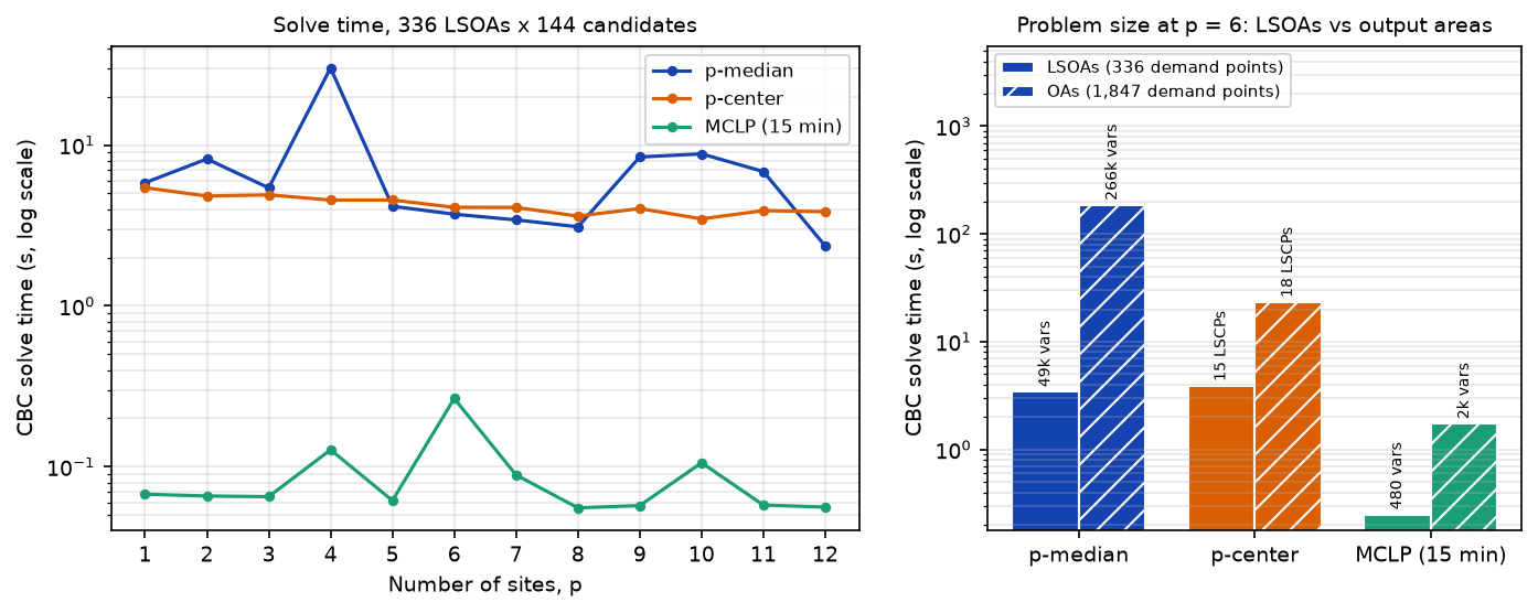
- p-median grows fastest. Five and a half times more demand points means five and a half times more variables and more than 50 times the solve time (185 seconds against 3.4), for the same answer: both solutions score identically on output-area demand. LSOAs lose nothing here because each LSOA’s population-weighted centroid already sits where its residents live.
- Solve time is erratic. The p-median at p = 4 took 30 seconds, five to seven times longer than at p = 3 or 5, with the same model size. Branch and bound can be lucky or unlucky; do not extrapolate from a single run.
- MCLP and LSCP scale gently, because they have one variable per site and per demand point, not per pair.
For bigger problems, such as all of England’s LSOAs, reduce the candidates first (as thin() does), drop demand–site pairs beyond a sensible maximum time, try a faster solver through PuLP (HiGHS is free; Gurobi and CPLEX have academic licences), or use a heuristic such as the Teitz–Bart vertex substitution, which gives very good p-median solutions quickly without a proof of optimality.
Step 6: adding sites to the existing network
New sites are rarely placed on a blank map. spopt’s predefined_facilities_arr forces chosen columns to be open. Put the 12 hospital sites first in the matrix, fix them, and ask for 15 sites in total, so the model chooses the best three additions:
T_ext = np.hstack([T_h, T]) # 12 hospital columns, then 144 candidatesfixed = np.arange(T_h.shape[1])for k in ("p-median", "mclp"): opened, secs, status, *_ = solve(k, len(hosp) + 3, M=T_ext, predefined=fixed)p-median Optimal in 2.6 s | mean 6.5 min (was 7.6) | worst 26.1 min (was 26.1) | 97.5% within 15 min (was 90.7%) | new: Isambard House; Wadebridge Town Hall; Wilcove Village Hallmclp Optimal in 0.1 s | mean 6.6 min (was 7.6) | worst 26.1 min (was 26.1) | 98.6% within 15 min (was 90.7%) | new: Wadebridge Town Hall; Downderry and Seaton Village Hall; Callington Town Hall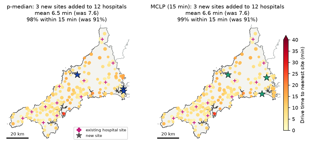
Both models choose Wadebridge, on the Camel estuary between Bodmin and Padstow, and both add sites in south-east Cornwall, which the hospital network serves only from Liskeard. Three well-chosen additions raise the share of residents within 15 minutes from 90.7% to 97.5% (p-median) or 98.6% (MCLP), and cut the mean from 7.6 to about 6.5 minutes.
Two results are a warning about the inputs, not about the models. First, p-median puts a site at Wilcove, near Torpoint. Torpoint looks remote in the road network because its ferry to Plymouth is not a road, and Plymouth’s Derriford Hospital is not in the model, so the model’s answer depends on what the network and the candidate list leave out. Second, the worst case does not change (26.1 minutes) because neither model cares about it: the worst-served LSOA, on the Roseland peninsula, is across the water from Falmouth but a long drive round the Fal estuary. A p-center model with the hospitals fixed would target it.
Limitations and honest caveats
These models are a planning aid: they make the consequences of an objective explicit and are good at finding options people had not considered. They do not make the decision.
- Free-flow car times. As in Part 1, travel times assume speed limits and no congestion, parking or junction delay, and car access. For urgent care, many patients arrive by ambulance, bus or a lift. A public transport matrix from r5py would change the answer.
- Ferries and the study boundary. The drive network leaves out the Torpoint and King Harry ferries, and the models ignore services in Devon and Plymouth. Include out-of-area facilities as fixed sites if people really use them, as Part 1 showed for GP practices.
- No capacity. All three models assume any site can serve any number of people. A capacitated p-median, or a check of demand per site after solving, is needed if sites have limited staff or rooms.
- Candidate quality. OpenStreetMap’s community buildings are a convenient list of real places, but not a list of buildings that are available, accessible or big enough. In practice the candidates should come from the estates team.
- Demand is residents. Census residents leave out Cornwall’s large summer population, which adds most demand for urgent care where it is most seasonal. The hospital list is from OSM and not an official list of urgent treatment centres.
- Aggregation (MAUP). Each LSOA’s residents are put at one point. Step 5 found the same p-median sites with output areas, but coverage results near the 15-minute threshold are sensitive to where those points sit.
- Ties and multiple optima. Several site sets can share the optimal objective, especially for p-center. Treat the chosen sites as one good answer, and look at the sites that keep coming up across models and values of p.
Frequently asked questions
What is location-allocation?
Location-allocation is a family of optimisation models that choose where to put a set of facilities and which demand each facility serves. The inputs are demand points with weights, such as population, candidate sites, and a travel-cost matrix between them. The model picks the sites that optimise an objective: the least total travel (p-median), the least worst travel (p-center), the most demand within a standard (maximal covering), or the fewest sites to cover everyone (set covering).
How do I solve the p-median problem in Python?
Build a NumPy matrix of travel costs from demand points (rows) to candidate sites (columns) and a vector of demand weights, then run PMedian.from_cost_matrix(cost, weights, p_facilities=p).solve(pulp.PULP_CBC_CMD(msg=False)) from spopt.locate. The open sites are those whose fac2cli list is not empty. spopt also has from_geodataframe constructors that compute Euclidean distances, but road-network times are more realistic, as in Step 2.
What is the difference between p-median, p-center and the maximal covering location problem?
p-median minimises the total, or average, demand-weighted travel cost: it is efficient but can leave remote places far from a site. p-center minimises the largest travel cost to any demand point: it is fair to the worst-off but ignores how many people benefit. The maximal covering location problem (MCLP) maximises the demand within a service standard, such as 15 minutes, and ignores how far beyond it anyone is. In this tutorial they chose six completely different sets of six sites.
Which solver should I use with spopt?
Any solver that PuLP supports. CBC comes with PuLP, so pulp.PULP_CBC_CMD() works with no extra installation, and it solved every model here. HiGHS (pulp.HiGHS() after pip install highspy) is free and often faster on large problems. Gurobi and CPLEX are commercial but have free academic licences. Set timeLimit, and check problem.sol_status as well as the status: a run stopped by the time limit returns its best solution so far, which may not be optimal.
Why is my p-center or p-median model slow?
The p-median and p-center models have one variable per demand–site pair, so they grow with the product of the two. Reduce the problem: aggregate demand to larger areas, thin or pre-filter the candidate sites, or remove pairs that are too far apart to matter. For p-center, solve a sequence of location set covering problems (LSCP) and bisect on the radius, as in Step 5; here that cut the solve time from over two minutes to about four seconds.
How many facilities do I need?
The models do not decide p for you. Solve for a range of p and plot the trade-off curves, as in Step 4, to show what each extra site buys. If you have a firm standard, such as “everyone within 20 minutes”, the location set covering problem (LSCP) gives the minimum number of sites needed to meet it.
Next steps
- If you have not already, read Part 1: the two-step floating catchment area (2SFCA) in Python, which builds the drive network and measures how access to GP practices varies across Cornwall today.
- Learn more about drive networks, routes and isochrones in street network analysis with OSMnx.
- Check whether the poorly served areas cluster with hot spot analysis in Python.
- Join the results to other area data with spatial joins in GeoPandas.
Data and licences
- Population: ONS, Census 2021 TS001: number of usual residents in households and communal establishments, from Nomis. Contains public sector information licensed under the Open Government Licence v3.0.
- Centroids and boundaries: ONS, LSOA (December 2021) Population Weighted Centroids (V4), Output Areas (December 2021) Population Weighted Centroids (V4), Output Areas (2021) Boundaries EW BGC (V2) and Local Authority Districts (May 2026) Boundaries UK BGC, from the Open Geography Portal. Source: Office for National Statistics licensed under the Open Government Licence v3.0. Contains OS data © Crown copyright and database right 2026.
- Roads, community buildings and hospitals: © OpenStreetMap contributors, available under the Open Database Licence. Cornwall and Devon extracts from Geofabrik, downloaded on 27 October 2026.
- Software: spopt (PySAL, BSD 3-Clause) and PuLP with the CBC solver (EPL 2.0).
Key terms
- Location-allocation
- Choosing where to put facilities (location) and which demand each facility serves (allocation) together, to optimise an objective such as total travel time or coverage.
- p-median problem
- Choose p facilities to minimise the total demand-weighted travel cost, with each demand point served by its nearest open facility (Hakimi, 1964; ReVelle and Swain, 1970). It is the efficiency model.
- p-center problem
- Choose p facilities to minimise the largest travel cost from any demand point to its nearest open facility. It is the equity, or worst-case, model and ignores how many people live where.
- Maximal covering location problem (MCLP)
- Choose p facilities to maximise the demand within a service standard, such as 15 minutes, of at least one open facility (Church and ReVelle, 1974). Demand beyond the standard counts for nothing, however far away it is.
- Location set covering problem (LSCP)
- Find the fewest facilities needed so that every demand point is within a given service standard of at least one of them (Toregas and others, 1971).
- Integer linear programme
- An optimisation problem with a linear objective and linear constraints in which some variables must be whole numbers, such as 0 or 1 for 'open this site or not'. Solvers such as CBC use branch and bound to find the proven optimum.
Data for this tutorial
- Nomis · Census 2021 table TS001 (usual residents) by LSOA and output area
- Open Geography Portal · ONS 2021 LSOA and output area population-weighted centroids, output area and local authority boundaries
- Geofabrik OpenStreetMap extract (England) · Cornwall and Devon .osm.pbf extracts for the drive network, community buildings and hospitals
Licences and formats for each source are listed in the GIS data sources catalogue.