Geodemographic classification in Python: k-means on Census 2021 Output Areas, and SKATER and max-p regionalisation

Short answer: to build a geodemographic classification in Python, download Census 2021 tables for Output Areas from Nomis, turn counts into percentages, transform skewed variables (the inverse hyperbolic sine, np.arcsinh, works well), standardise them to z-scores, drop near-duplicate variables, and run scikit-learn’s KMeans with many random starts. Choose k from the elbow, the silhouette and stability across seeds, together with how useful the clusters are, then profile them with index scores before you name them. If you need contiguous regions rather than area types, use spopt’s Skater or MaxPHeuristic on a queen contiguity graph. For Cardiff’s 1,115 Output Areas, seven k-means clusters explained 52% of the variance in 25 variables but fell into 157 separate pieces; seven SKATER regions explained 34%.

Geodemographic classifications sort neighbourhoods into types such as “student quarter” or “detached owner-occupier suburbs”. The UK has an official one, the 2021/2 Output Area Classification (OAC), and commercial ones such as Acorn and Mosaic. Building your own is useful when you want one city, different variables or a different purpose, and doing it once is the best way to learn how much the official product depends on judgement. This tutorial builds a small classification of Cardiff with real Census 2021 data and is explicit about every judgement it makes.

You will learn how to:

1. download Census 2021 tables for Output Areas from Nomis and build 27 candidate variables;
2. transform and standardise them, and check correlations to remove duplicates;
3. choose k for k-means with the elbow, the silhouette and stability across random seeds;
4. profile the clusters with index scores, a heatmap and radar charts, and name them cautiously;
5. compare the result with the official 2021/2 OAC and see the MAUP at work at LSOA level;
6. build contiguous regions with SKATER and max-p in spopt, and decide when you want contiguity.

Setup

The full script, geodemographic_classification.py, runs from top to bottom and writes seven figures, a GeoPackage and a JSON file of metrics to output/. It caches downloads in data/. Install the tested versions with:

pip install scikit-learn==1.9.1 spopt==0.8.0 libpysal==4.15.1 networkx==3.7 geopandas==1.2.0 shapely==2.2.0 pyogrio==0.13.0 pyproj==3.8.0 numpy==2.5.4 pandas==3.1.0 scipy==1.18.1 matplotlib==3.11.2 requests==2.34.2

The whole script takes about eight minutes on a laptop, almost all of it in max-p (Step 8). Everything else takes about a minute.

Step 1: Output Areas for Cardiff

Output Areas (OAs) are the smallest areas with published Census 2021 results. Cardiff has 1,115 of them, grouped into 218 LSOAs. The ONS Open Geography Portal serves the boundaries through an ArcGIS REST service; LSOA names start with the local authority name, so a LIKE filter selects Cardiff.

OA_URL = f"{ONS}/Output_Areas_2021_EW_BGC_V2/FeatureServer/0/query"
feats, offset = [], 0
while True:
    page = requests.get(OA_URL, params={"where": "LSOA21NM LIKE 'Cardiff %'", "outFields": "OA21CD,LSOA21CD,LSOA21NM",
                                        "outSR": 27700, "f": "geojson", "resultOffset": offset,
                                        "resultRecordCount": 1000}, timeout=300).json()
    feats += page["features"]; offset += len(page["features"])
    if len(page["features"]) < 1000:
        break

1,115 Output Areas in 218 LSOAs, 142.3 km2

Step 2: Census 2021 variables from Nomis

Nomis publishes every Census 2021 topic summary table as a bulk zip with one CSV per geography level, so a single download gives you all 188,880 OAs in England and Wales. The script downloads 15 tables, keeps Cardiff’s OAs, and turns counts into percentages of the right base: people for age and ethnicity, households for tenure and cars, residents aged 16 and over for occupation and qualifications.

NOMIS = "https://www.nomisweb.co.uk/output/census/2021/census2021-{}.zip"

def table(code):
    z = zipfile.ZipFile(download(NOMIS.format(code), DATA / f"census2021-{code}.zip"))
    df = pd.read_csv(z.open(f"census2021-{code}-oa.csv")).set_index("geography code")
    df.columns = [c.split(": ", 1)[1].replace("; measures: Value", "") if ": " in c else c for c in df.columns]
    return df.loc[oa.OA21CD]

def pct(df, num, den):
    num = [num] if isinstance(num, str) else num
    return 100 * df[num].sum(axis=1) / df[den]

age, hh, ten = table("ts007a"), table("ts003"), table("ts054")
# ... 12 more tables

V = pd.DataFrame(index=oa.OA21CD)
V["Aged 65+"] = pct(age, ["Aged 65 to 69 years", "Aged 70 to 74 years", "Aged 75 to 79 years",
                         "Aged 80 to 84 years", "Aged 85 years and over"], "Total")
V["Social rented"] = pct(ten, "Social rented", "Total: All households")
V["Full-time students"] = pct(sec, "L15 Full-time students", sec_tot)
V["Born outside UK"] = 100 - pct(cob, "Europe: United Kingdom", "Total")
V["Welsh speakers"] = pct(welsh, [c for c in welsh.columns if c.startswith("Can speak")],
                          "Total: All usual residents aged 3 years and over")
# ... 22 more variables

The 27 candidates cover the themes that most classifications use: age, household type, tenure, housing type, overcrowding, cars, occupation (NS-SeC), qualifications, unemployment, health, ethnicity, country of birth, plus population density and, because this is Wales, the share of people who can speak Welsh.

27 candidate variables for 1,115 OAs; 0 missing values
Cardiff: 362,289 usual residents; OA population median 313, range 101-1730
                         mean     50%   min      max
Aged 20-24                9.3     5.6   0.0     79.4
Aged 65+                 15.4    13.6   0.0     91.1
Population density     7135.5  5802.5  53.9  47887.3
Social rented            17.1     7.2   0.0     91.1
Detached                 14.4     4.3   0.0     98.4
Flats                    25.5    15.1   0.0    100.0
Full-time students       12.4     7.4   0.0     95.2
Unemployed                2.9     2.6   0.0     37.2
Black                     3.7     2.2   0.0     51.0
Welsh speakers           12.3    11.1   0.0     47.0

Step 3: transform, standardise and check correlations

The variables are on very different scales (density runs to 47,887 people per km², the percentages to 100) and many are skewed: most OAs have few students or Black residents, and a few have a lot. Without treatment, k-means would be dominated by density and by a handful of extreme OAs. The script applies the inverse hyperbolic sine, which behaves like a logarithm but is defined at zero, then converts every variable to a z-score (mean 0, standard deviation 1).

T = np.arcsinh(V)                       # inverse hyperbolic sine: log-like, but defined at zero
Z = (T - T.mean()) / T.std(ddof=0)      # z-scores
C = Z.corr()
pairs = [(a, b, C.loc[a, b]) for i, a in enumerate(C) for b in C.columns[i + 1:] if abs(C.loc[a, b]) >= 0.8]

DROP = ["Degree level (L4+)", "Owns with mortgage"]
Zk = Z.drop(columns=DROP)
X = Zk.to_numpy()

median |skewness|: raw 1.38 -> IHS 0.59; most skewed raw: Unemployed 4.4, Black 3.5, Aged 20-24 3.4
|r| >= 0.8: Higher professional ~ Degree level (L4+): r = 0.88
|r| >= 0.8: Routine occupations ~ No qualifications: r = 0.87
|r| >= 0.8: No qualifications ~ Bad health: r = 0.81
|r| >= 0.8: Aged 20-24 ~ Full-time students: r = 0.80
dropping ['Degree level (L4+)', 'Owns with mortgage']: degree level duplicates higher professional (r = 0.88); the four tenure shares sum to ~100%, so one is redundant
25 variables go into the clustering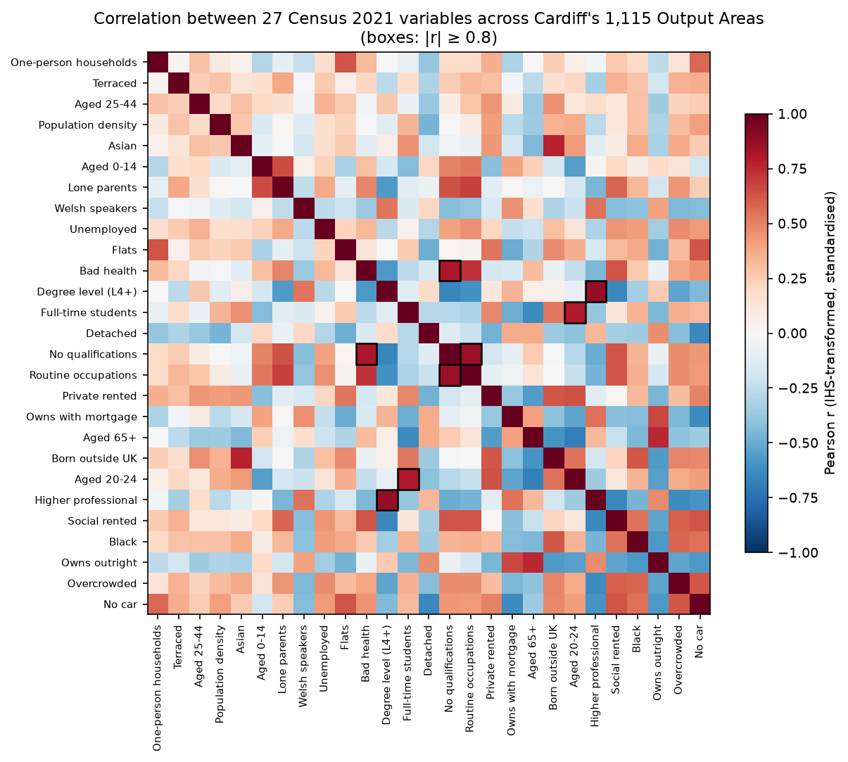

Correlation of 0.8 or more is a common rule of thumb for “measuring the same thing”. We dropped degree-level qualifications, which is almost the same signal as higher professional occupations, and owning with a mortgage, because the four tenure shares add up to 100% and any one is implied by the others. We kept the other three pairs: routine occupations, no qualifications and bad health overlap but are not the same concept, and students and 20–24-year-olds diverge in places with young workers. These are judgements, and a different analyst could defend different ones.

Step 4: choosing k

k-means needs the number of clusters in advance. Three diagnostics help, and none of them decides on its own:

• the elbow: the within-cluster sum of squares falls as k grows; look for a bend after which extra clusters help little;
• the mean silhouette: how much closer areas are to their own cluster than to the next nearest one;
• stability: whether k-means finds the same solution from different random starts, measured with the adjusted Rand index (ARI).

for k in range(2, 13):
    km = KMeans(k, n_init=50, random_state=SEED).fit(X)
    print(k, km.inertia_, silhouette_score(X, km.labels_))

for k in (4, 5, 6, 7, 8, 9):
    runs = [KMeans(k, n_init=1, random_state=s).fit(X).labels_ for s in range(30)]
    best = KMeans(k, n_init=100, random_state=SEED).fit(X).labels_
    vs_best = np.median([adjusted_rand_score(best, r) for r in runs])
    pairwise = np.mean([adjusted_rand_score(runs[i], runs[j]) for i in range(30) for j in range(i + 1, 30)])

k= 2: within-cluster sum of squares    21192 | silhouette 0.224
k= 3: within-cluster sum of squares    17401 | silhouette 0.241
k= 4: within-cluster sum of squares    15966 | silhouette 0.217
k= 5: within-cluster sum of squares    14763 | silhouette 0.169
k= 6: within-cluster sum of squares    13916 | silhouette 0.154
k= 7: within-cluster sum of squares    13286 | silhouette 0.161
k= 8: within-cluster sum of squares    12873 | silhouette 0.144
k= 9: within-cluster sum of squares    12474 | silhouette 0.128
k=10: within-cluster sum of squares    12152 | silhouette 0.130
k=11: within-cluster sum of squares    11856 | silhouette 0.122
k=12: within-cluster sum of squares    11550 | silhouette 0.116
k=4: 30 single-start runs vs the 100-start solution, median ARI 0.416; mean pairwise ARI 0.787
k=5: 30 single-start runs vs the 100-start solution, median ARI 0.959; mean pairwise ARI 0.833
k=6: 30 single-start runs vs the 100-start solution, median ARI 0.728; mean pairwise ARI 0.698
k=7: 30 single-start runs vs the 100-start solution, median ARI 0.708; mean pairwise ARI 0.710
k=8: 30 single-start runs vs the 100-start solution, median ARI 0.649; mean pairwise ARI 0.628
k=9: 30 single-start runs vs the 100-start solution, median ARI 0.641; mean pairwise ARI 0.613
chosen k = 7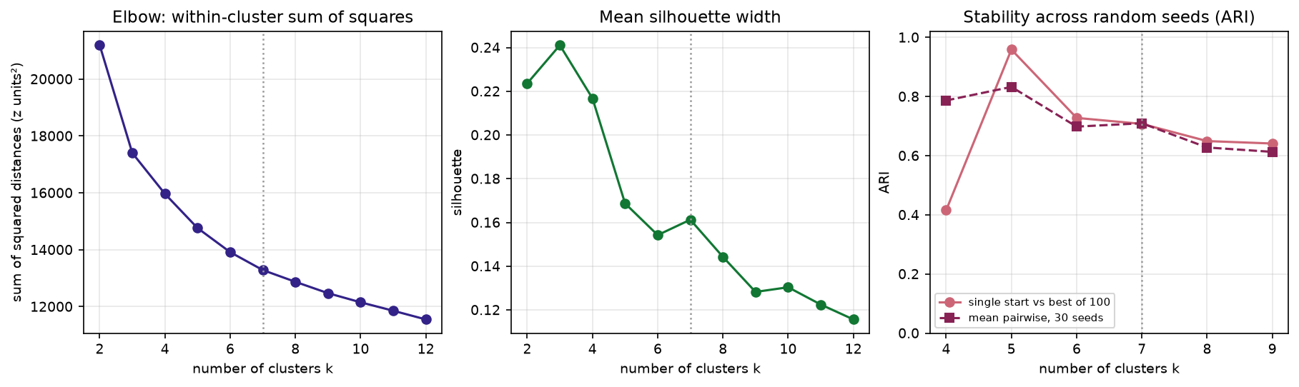

This is a typical result for census data, and it is worth being honest about. There is no clear elbow. The silhouette is highest at k = 3, but three clusters (roughly “affluent suburbs”, “deprived estates” and “inner city”) are too coarse to be useful. Census variables vary continuously across a city, so clusters are convenient divisions of a continuum rather than natural groups, and silhouette values of 0.1–0.25 are normal.

We chose k = 7. It has a small local peak in the silhouette and separates two groups that matter in Cardiff and merge at lower k: the student quarter and city-centre renters in flats. k = 5 was the most stable choice and would be a defensible alternative. Single-start runs at k = 7 agreed with the 100-start solution only moderately (median ARI 0.708), which is why the final model uses n_init=100. Always use many starts for the final run.

Step 5: profile the clusters and name them cautiously

The final model takes the best of 100 starts. To describe each cluster in units people understand, the script computes index scores from the untransformed percentages: the cluster’s rate (weighted by residents) divided by the Cardiff rate, times 100.

km = KMeans(7, n_init=100, random_state=SEED).fit(X)
s = silhouette_samples(X, oa.kmeans)

city = V.mul(residents, axis=0).sum() / residents.sum()
idx = pd.DataFrame({c: V[oa.kmeans.to_numpy() == c].mul(residents[oa.kmeans == c], axis=0).sum()
                    / residents[oa.kmeans == c].sum() for c in range(K)}).T
index = (100 * idx / city).round(0)

k = 7: mean silhouette 0.161; OAs with negative silhouette 5.3%
cluster 0 (250 OAs, 82,074 people): high Social rented 252, Lone parents 220, No qualifications 178, Routine occupations 171 | low Detached 33, Higher professional 37, Degree level (L4+) 54
cluster 1 (241 OAs, 77,080 people): high Detached 301, Owns outright 174, Higher professional 168, Aged 65+ 159 | low Social rented 11, Black 19, Flats 21
cluster 2 (188 OAs, 53,202 people): high Aged 65+ 160, Owns outright 137, Bad health 124, One-person households 116 | low Black 33, Full-time students 36, Aged 20-24 42
cluster 3 (160 OAs, 54,194 people): high Population density 294, Black 244, Asian 211, Born outside UK 190 | low Detached 24, Aged 65+ 56, Owns outright 59
cluster 4 (160 OAs, 50,693 people): high Terraced 162, Higher professional 150, Welsh speakers 142, Degree level (L4+) 136 | low Social rented 33, Overcrowded 51, Black 56
cluster 5 (58 OAs, 15,124 people): high Flats 348, Private rented 253, Born outside UK 195, Aged 25-44 187 | low Detached 4, Lone parents 24, Social rented 30
cluster 6 (58 OAs, 29,922 people): high Full-time students 506, Aged 20-24 459, Population density 287, Private rented 253 | low Detached 17, Aged 0-14 19, Aged 65+ 21

The console numbers clusters from 0, ordered by size; the figures and the names add one. The heatmap shows all 27 index scores, including the two variables that were not used in the clustering.

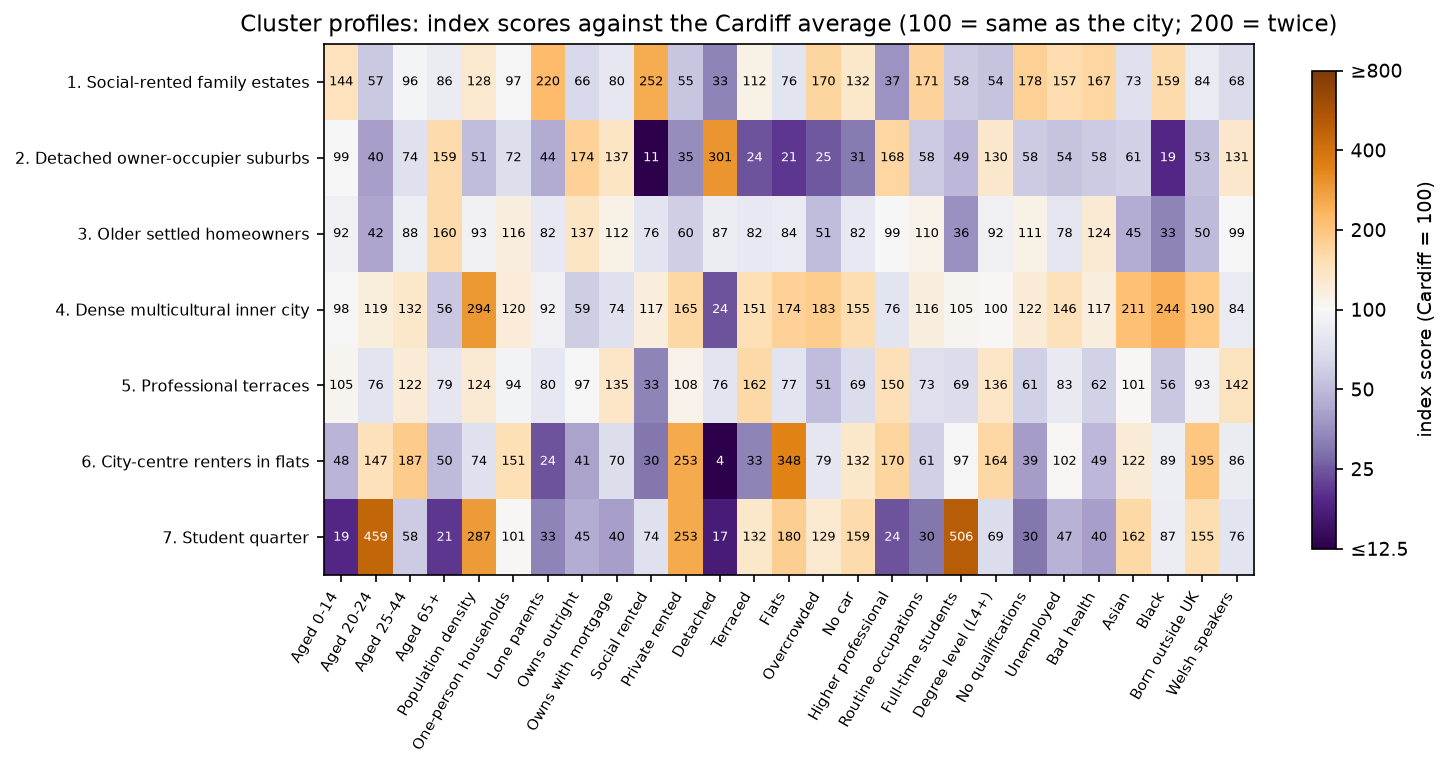
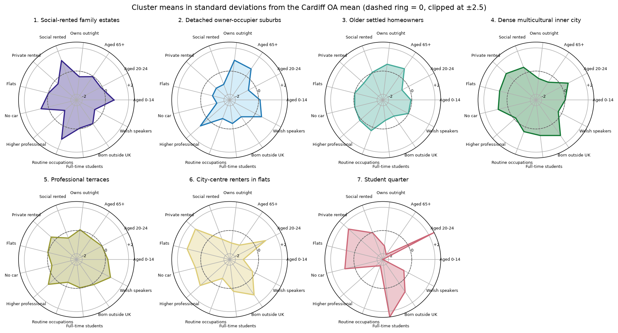
We named the clusters only after reading these profiles:

1. Social-rented family estates (250 OAs): 2.5 times the city’s share of social renting and 2.2 times its share of lone-parent households.
2. Detached owner-occupier suburbs (241 OAs): three times the share of detached houses; very little social renting.
3. Older settled homeowners (188 OAs): more people aged 65+, outright owners and people in bad health.
4. Dense multicultural inner city (160 OAs): about three times the city’s density and twice its shares of Black and Asian residents.
5. Professional terraces (160 OAs): terraced housing, professional occupations and the highest share of Welsh speakers.
6. City-centre renters in flats (58 OAs): 3.5 times the share of flats, 2.5 times the share of private renting, many people aged 25–44.
7. Student quarter (58 OAs, almost 30,000 people): five times the city’s share of full-time students.

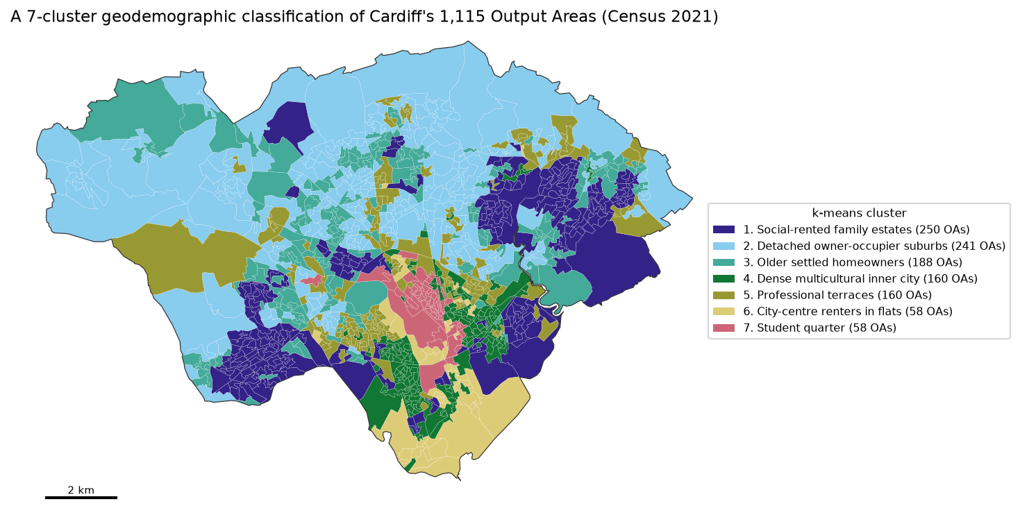
The map shows the main property of a classification: areas of the same type need not be next to each other. Social-rented family estates appear in the east and the south-west, and professional terraces appear in several inner suburbs. The silhouette also tells you which areas fit badly: 5.3% of OAs are closer, on average, to another cluster than to their own. They are worth listing and checking on the ground before anyone uses the classification for decisions.

Step 6: compare with the official 2021/2 OAC

The UK has an official classification. The 2021/2 Output Area Classification, built by UCL and the ONS and published by the Geographic Data Service, assigns every OA in the UK to one of 8 supergroups, 21 groups and 52 subgroups using 60 census variables, the inverse hyperbolic sine and k-means: broadly the same recipe as this tutorial, at national scale. It is the reference product to use when you need a classification that is comparable across the UK. The script downloads it and cross-tabulates our clusters against its supergroups.

oac = pd.read_csv(download(OAC_URL, DATA / "uk_oac_final.csv"), dtype=str).set_index("GeographyCode")
oa["oac_sg"] = oac.Supergroup.reindex(oa.OA21CD).to_numpy()
print(adjusted_rand_score(oa.oac_sg, oa.kmeans))
print(pd.crosstab(oa.kmeans, oa.oac_sg))

matched 1115 of 1115 OAs to the official classification
official supergroups in Cardiff: 1 Retired Professionals 111; 2 Suburbanites and Peri-Urbanites 113; 3 Multicultural and Educated Urbanites 139; 4 Low-Skilled Migrant and Student Communities 141; 5 Ethnically Diverse Suburb-an Professionals 182; 6 Baseline UK 374; 7 Semi- and Un-Skilled Workforce 44; 8 Legacy Communities 11
ARI between our k-means and the official supergroups (8 classes, UK-wide): 0.282
ARI against the official groups (21 present): 0.323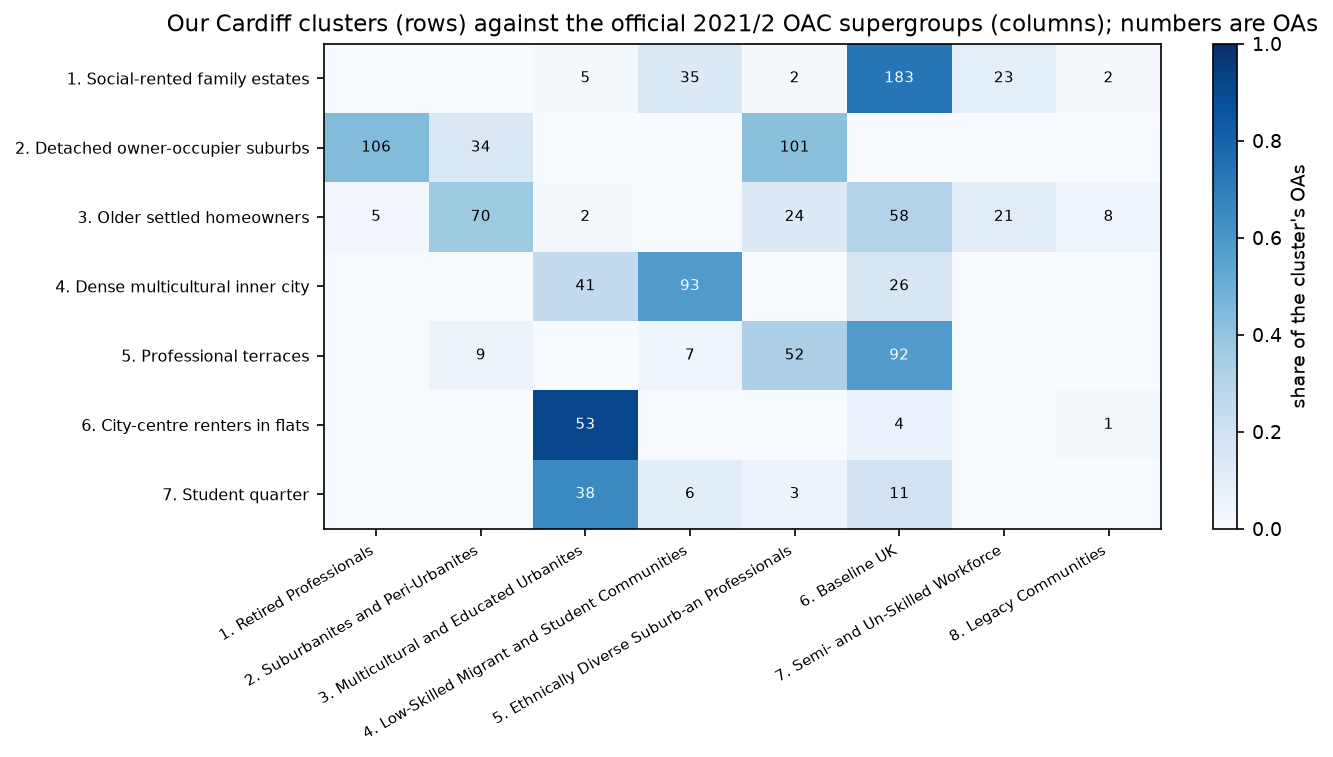

The two classifications agree in broad terms but are far from identical (ARI 0.282 against supergroups, 0.323 against groups). That is expected. The OAC was built for the whole UK, so its clusters describe differences between places such as rural Wales, inner London and Cardiff; within one city, a UK-wide type such as “Baseline UK” (374 of Cardiff’s OAs) can hide differences that matter locally. Our classification was built only on Cardiff, so its types are relative to Cardiff. Some differences are also instructive: our “Student quarter” is mostly in the OAC’s “Multicultural and Educated Urbanites” supergroup (38 of 58 OAs) rather than its “Low-Skilled Migrant and Student Communities”, which in Cardiff matches our dense inner-city cluster better. Neither classification is wrong; they answer different questions.

Step 7: the MAUP: what changes at LSOA level?

Geodemographic results depend on the zones you use, which is one form of the modifiable areal unit problem (MAUP). To see how much, the script aggregates the same variables to Cardiff’s 218 LSOAs (population-weighted means of the OA percentages, which approximate the LSOA rates) and repeats the whole recipe.

VL = V.drop(columns="Population density").mul(residents, axis=0).groupby(lsoa_key).sum().div(
    pd.Series(residents).groupby(lsoa_key).sum().to_numpy(), axis=0)
TL = np.arcsinh(VL[V.columns].drop(columns=DROP))
ZL = ((TL - TL.mean()) / TL.std(ddof=0)).to_numpy()
lab_l = KMeans(7, n_init=100, random_state=SEED).fit(ZL).labels_
oa_from_lsoa = pd.Series(lab_l, index=VL.index).reindex(lsoa_key).to_numpy()

218 LSOAs, k = 7: silhouette 0.212; ARI with the OA classification (each OA takes its LSOA's cluster) 0.416
LSOAs whose OAs fall in more than one OA-level cluster: 70%; max-min range of 'Full-time students' within LSOAs, median 5.9 points

The LSOA classification has a higher silhouette (0.212 against 0.161), but that does not make it better: averaging over about five OAs smooths away the variation that makes OAs hard to separate. The two classifications agree only moderately (ARI 0.416), and 70% of LSOAs contain OAs from more than one OA-level cluster. Use the smallest zones your data support, report the zone you used, and do not apply a classification built for one geography to another without checking.

Step 8: contiguous regions with SKATER and max-p

A classification answers “what kind of place is this?” A regionalisation answers a different question: “how should I divide this city into a few internally similar, connected regions?” Each region must be a single contiguous piece. You want contiguity when the result will be used as a set of areas, for example:

• reporting or service areas, such as neighbourhood management areas, catchments or sales territories, which must be contiguous to be managed;
• zones for small-area statistics, where max-p’s population floor guarantees that every region has enough people for stable rates and for disclosure control;
• sampling frames and survey strata that fieldworkers can cover area by area;
• spatial analysis that needs areas of similar size, to reduce the effect of very small or very large zones.

You do not want contiguity when you are targeting a type of area (a leaflet campaign to every student area, for instance) or comparing like with like across a city: a classification lets similar areas be far apart, and a contiguity constraint would force unlike areas together.

spopt, the regionalisation module of PySAL, provides SKATER, max-p, AZP and others. They all need a spatial weights object that says which OAs touch. The script uses queen contiguity (sharing an edge or a corner) and checks that the graph is connected, because an island with no neighbours can never join a region.

w = libpysal.weights.Queen.from_dataframe(oa, use_index=False, silence_warnings=True)
attrs = list(Zk.columns)
reg = oa[["geometry"]].copy()
reg[attrs] = X                                     # the same 25 standardised variables as k-means
reg["residents"] = residents

sk = Skater(reg, w, attrs, n_clusters=7, floor=20, trace=False, islands="increase")
sk.solve()

np.random.seed(SEED); random.seed(SEED)           # max-p's heuristic is randomised
mp = MaxPHeuristic(reg, w, attrs, "residents", 20_000, top_n=2, max_iterations_construction=50)
mp.solve()

SKATER builds a minimum spanning tree of the contiguity graph, with edge costs equal to the attribute dissimilarity between neighbours, and then cuts the tree into k pieces, choosing the cuts that most reduce within-region variation. Here we ask for seven regions with at least 20 OAs each. max-p works the other way round: you set a floor on a spatially extensive variable (here, at least 20,000 residents per region) and it finds the largest number of regions that meets the floor, then improves their homogeneity by moving OAs between regions. AZP (spopt.region.AZP) is a similar local-search alternative when you want a fixed number of regions.

queen contiguity: mean 6.0 neighbours, islands 0, connected components 1
SKATER with 7 regions, floor 20 OAs: 2.0 s; region sizes (OAs) [399, 242, 141, 129, 108, 53, 43]
max-p, every region >= 20,000 residents: p = 16 regions in 411.0 s; region populations 20,025-26,734

To compare the three results, the script computes the share of the variance in the 25 standardised variables that each grouping explains (1 − within-group sum of squares ÷ total sum of squares, an R²), and counts the contiguous pieces each grouping makes on the map.

k-means (no contiguity) :  7 groups | share of variance explained 0.523 | contiguous pieces on the map 157
SKATER                  :  7 groups | share of variance explained 0.344 | contiguous pieces on the map 7
max-p                   : 16 groups | share of variance explained 0.464 | contiguous pieces on the map 16
ARI k-means vs SKATER 0.266; k-means vs max-p 0.205
for reference, aspatial k-means with k = 16 explains 0.614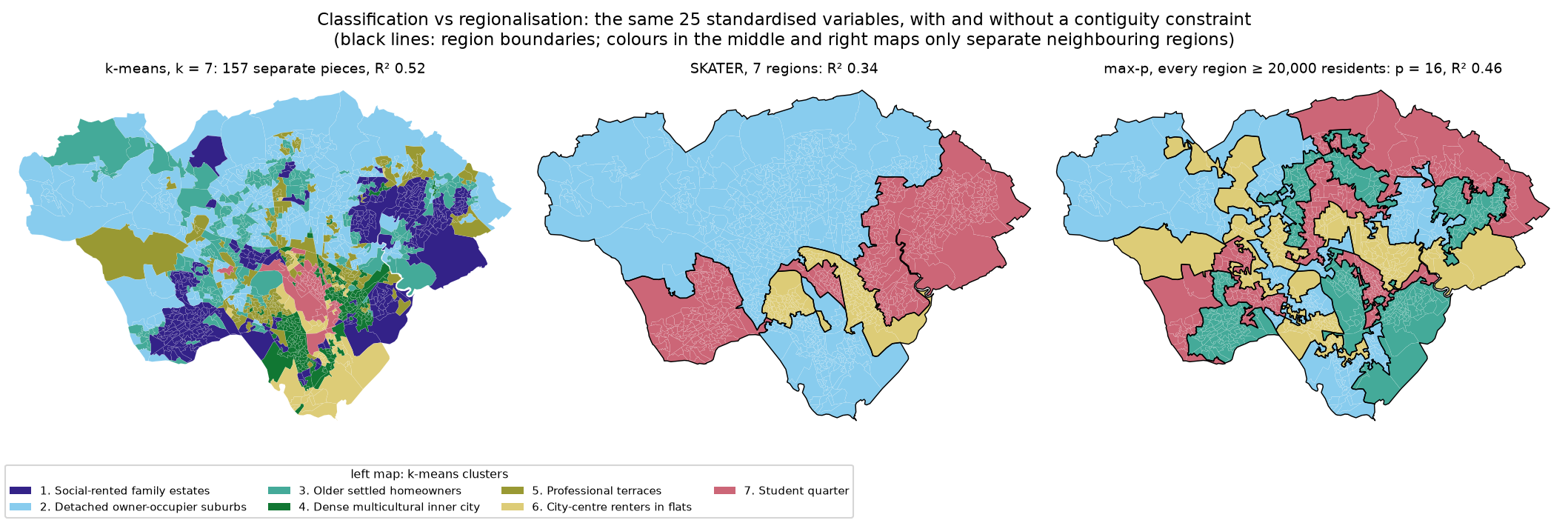

The contiguity constraint has a clear cost. With seven groups, SKATER explains 34% of the variance against 52% for k-means, because each region must include whatever lies between its similar areas. SKATER’s regions are also very unequal (399 OAs in the largest, 43 in the smallest), since it cuts the tree wherever that helps homogeneity most. max-p’s regions are more even by design (20,025–26,734 residents each), and its 16 regions explain 46% of the variance, against 61% for 16 unconstrained k-means clusters. In return you get areas you can draw, name and manage.

Limitations and honest caveats

• Census 2021 was taken during the COVID-19 pandemic. On 21 March 2021 some students were living at their family homes rather than at university, so student areas in Cardiff may be under-represented, and some people’s occupations and travel were affected by furlough and lockdown rules.
• The variables decide the result. Different variables, or a different balance between themes, would give different clusters. The 27 candidates here are a reasonable small set, not a standard.
• k is a choice. The diagnostics did not agree, and k = 5 would have been equally defensible. Report the alternatives you considered.
• Clusters are averages. The ecological fallacy applies: a cluster’s profile does not describe every person, household or even every OA in it, and 5.3% of OAs fit their cluster poorly.
• Index scores need context. An index of 500 for a variable with a city rate of 1% means 5%; always show rates alongside index scores when it matters.
• Census statistics have small-number noise. The ONS applies targeted record swapping and cell key perturbation to protect confidentiality, so very small counts in single OAs are less reliable than the totals.
• The MAUP does not go away. The results depend on the OA boundaries; a classification of LSOAs or of a grid would differ.
• Regionalisation results depend on the parameters. SKATER’s floor and number of regions, and max-p’s threshold, are choices; so is queen rather than rook contiguity.

Frequently asked questions

How do I do k-means clustering on census data in Python?

Turn counts into percentages of a suitable base, transform skewed variables (for example with np.arcsinh), standardise every variable to z-scores, drop near-duplicates, and fit sklearn.cluster.KMeans(k, n_init=100, random_state=42). Choose k with the elbow, the silhouette and stability across random seeds, then profile the clusters with index scores against the study-area average.

Why standardise variables before k-means?

k-means uses Euclidean distance, so a variable measured on a larger scale, such as population density in thousands per km², would dominate percentages that range from 0 to 100. Converting each variable to a z-score gives every variable the same weight. Transforming skewed variables first (log, square root or inverse hyperbolic sine) stops a few extreme areas from dominating the standard deviation.

What is the difference between classification and regionalisation?

A classification groups areas by similarity only, so areas of the same type can be anywhere in the city. A regionalisation adds a contiguity constraint, so each group is one connected region. Use a classification to describe and target types of neighbourhood, and a regionalisation when you need a set of areas to manage, report on or sample from.

Should I use SKATER or max-p?

Use SKATER when you know how many regions you want and need a fast result; it can produce very unequal regions. Use max-p when every region must reach a minimum size, such as a population floor for stable rates or disclosure control, and you want the largest number of regions that meets it; it is randomised and much slower. AZP is a middle ground for a fixed number of regions.

Should I use the official OAC instead of building my own?

For most purposes, yes. The 2021/2 OAC covers the whole UK consistently, is documented and peer-reviewed, and is free under the Open Government Licence. Build your own when you need types relative to one city, variables the OAC does not use (such as the Welsh language here) or a classification for a specific purpose, and compare it with the OAC as in Step 6.

Can I use LSOAs instead of Output Areas?

Yes, and LSOAs are the only option for some data, such as the indices of deprivation. Expect smoother, more mixed clusters: in Cardiff, 70% of LSOAs contained OAs from more than one OA-level cluster, and the LSOA and OA classifications agreed only moderately (ARI 0.416).

Next steps

• Cluster points rather than areas, for example shops or GPS fixes, with our companion tutorial DBSCAN and HDBSCAN spatial clustering in Python.
• Build spatial weights in more depth and test whether a single variable is spatially clustered with hot spot analysis in Python (Getis-Ord Gi*).
• Relate two census variables to each other across small areas with bivariate correlation of census and crime data.
• Attach the clusters to points such as addresses or incidents with spatial joins in GeoPandas. The script writes output/cardiff_oa_classification.gpkg with the k-means, OAC, SKATER and max-p labels for every OA.
• Make publication-quality maps of the clusters with maps in Python with Matplotlib and Cartopy.

Data and licences

• Census 2021: Office for National Statistics, Census 2021 topic summary tables TS001, TS003, TS004, TS006, TS007A, TS021, TS032, TS037, TS044, TS045, TS052, TS054, TS062, TS066 and TS067 for Output Areas, bulk downloads from Nomis, downloaded on 27 October 2026. Source: Office for National Statistics licensed under the Open Government Licence v3.0.
• Boundaries: Office for National Statistics, Output Areas (December 2021) Boundaries EW BGC (V2), from the Open Geography Portal. Source: Office for National Statistics licensed under the Open Government Licence v3.0. Contains OS data © Crown copyright and database right 2026.
• 2021/2 Output Area Classification: Geographic Data Service / UCL and the Office for National Statistics, UK OAC v3.2 (January 2025), from data.geods.ac.uk, Open Government Licence v3.0. Reference: Wyszomierski, J., Longley, P. A., Singleton, A. D., Gale, C. and O’Brien, O. (2024), “A neighbourhood Output Area Classification from the 2021 and 2022 UK censuses”, The Geographical Journal 190(2): e12550.
• Further reading: Assunção, R. M., Neves, M. C., Câmara, G. and Freitas, C. da C. (2006), “Efficient regionalization techniques for socio-economic geographical units using minimum spanning trees”, International Journal of Geographical Information Science 20(7): 797–811 (SKATER); Duque, J. C., Anselin, L. and Rey, S. J. (2012), “The max-p-regions problem”, Journal of Regional Science 52(3): 397–419; Openshaw, S. (1984), The Modifiable Areal Unit Problem, CATMOG 38.
• Code: geodemographic_classification.py, tested with Python 3.12.0, scikit-learn 1.9.1, spopt 0.8.0, libpysal 4.15.1, networkx 3.7, geopandas 1.2.0, shapely 2.2.0, pyogrio 0.13.0, pyproj 3.8.0, numpy 2.5.4, pandas 3.1.0, scipy 1.18.1, matplotlib 3.11.2 and requests 2.34.2.