DBSCAN and HDBSCAN spatial clustering in Python: finding Glasgow's dining districts
Cluster GPS and point-of-interest data in Python with DBSCAN and HDBSCAN: use the haversine metric on latitude and longitude or plain metres on a projected grid, choose eps with a k-distance plot, handle variable density with HDBSCAN, draw convex and concave hull polygons, treat noise properly, read silhouette and DBCV with care, and scale up with a BallTree. Uses 3,950 real Overture Maps restaurants, cafés and bars in Glasgow.
- Level
- Intermediate
- Tested with
- Python 3.12
- Source code
- Download scripts
Key takeaways
- DBSCAN groups points that have at least min_samples neighbours within a radius eps, and labels everything else as noise. For latitude and longitude, pass [lat, lon] in radians with metric='haversine' and eps in metres divided by the Earth's radius (about 6,371 km). On a projected CRS in metres you can use the default Euclidean metric with eps in metres; for Glasgow the two gave the same 44 clusters (ARI 0.9994).
- The classic mistakes are silent. Passing eps=150 to the haversine metric put all 3,950 places in one cluster, because 150 radians is far more than half the planet. Running Euclidean DBSCAN on raw degrees gave 57 clusters instead of 44, because a degree of longitude is only 0.56 of a degree of latitude at 56° N.
- A k-distance plot gives a defensible eps. With min_samples = 10, the knee of the curve was at 171 m and the median distance to the 9th neighbour was 95 m, so eps = 150 m was a reasonable choice. A sensitivity grid shows how much the answer moves: from 120 to 9 clusters across eps 75–400 m and min_samples 5–30.
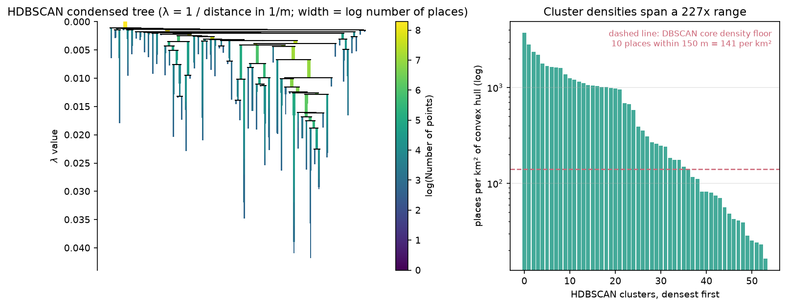
- One global eps cannot fit clusters whose densities differ by 227 times. DBSCAN chained the centre into one cluster of 1,205 places (31% of all of them). HDBSCAN, which needs only a minimum cluster size, split it into separate districts and found 54 clusters, 18 of them sparser than the density DBSCAN demands of a core point.
- Internal scores need care. HDBSCAN scored a silhouette of 0.516 and a DBCV of 0.193 against DBSCAN's 0.270 and −0.022, but HDBSCAN also found 28 'clusters' in uniformly random points (DBCV 0.096). Treat clusters of points of interest as a description, and check them against a null model and local knowledge.
Before you start
- Comfortable with GeoPandas and coordinate reference systems (see the GeoPandas getting-started and CRS tutorials)
- Python 3.10+ with scikit-learn 1.3+ (for sklearn.cluster.HDBSCAN), hdbscan, geopandas, shapely 2, duckdb, numpy, pandas, matplotlib and requests
- An internet connection: the first run reads about 4 MB of Overture Maps places from Amazon S3 with DuckDB and one ONS boundary
Short answer: to cluster GPS or point-of-interest data in Python, use scikit-learn’s DBSCAN. If your points are latitude and longitude, pass np.radians(df[["lat", "lon"]]) with metric="haversine" and set eps to a distance in metres divided by the Earth’s radius (6,371,008.8 m). If they are in a projected CRS in metres, such as British National Grid, use the default metric and set eps in metres. Choose eps from a k-distance plot. When clusters have very different densities, as they do in almost every city, switch to HDBSCAN, which needs only a minimum cluster size. For 3,950 restaurants, cafés and bars in Glasgow, DBSCAN with eps = 150 m merged the city centre into a single cluster of 1,205 places; HDBSCAN found 54 dining districts holding 72% of the places in 5.4% of the city’s area.
Density-based clustering is the usual answer to the question “where are the clusters?” for point data, because, unlike k-means, it does not need the number of clusters in advance, it finds clusters of any shape, and it can leave isolated points unclustered as noise. It is also easy to get subtly wrong. Units, the choice of eps, and the difference between “a cluster” and “an area where points happen to be dense” all matter. This tutorial uses real open data from Overture Maps and spends as much time on those choices as on the code.
You will learn how to:
- read restaurants, cafés and bars for one city from Overture Maps with DuckDB;
- run DBSCAN with the haversine metric on latitude and longitude in radians, and on projected metres, and see that they agree;
- choose eps with a k-distance plot, set min_samples, and test the sensitivity of the result;
- use HDBSCAN (
sklearn.cluster.HDBSCANand thehdbscanpackage) for clusters of variable density; - turn clusters into convex and concave hull polygons and handle the noise;
- report silhouette and DBCV scores with the caveats they need;
- scale to tens of thousands of points with a BallTree.
All outputs below are real results from dbscan_dining_districts.py, run on 27 October 2026 with Python 3.12.0, scikit-learn 1.9.1, hdbscan 0.8.44, geopandas 1.2.0, shapely 2.2.0 and DuckDB 1.5.6.
The data: Overture Maps places in Glasgow
Overture Maps publishes a global places theme of tens of millions of points of interest, built from Meta, Microsoft and other sources, as GeoParquet files on Amazon S3. Each place has a name, a category, a confidence score between 0 and 1, an operating status and, often, an address. We use Glasgow City, Scotland’s largest council area. It has a dense city centre, a West End with a well-known restaurant strip, a Southside with a different mix, and large residential schemes with few restaurants, so its clusters should vary in size and density.
The first step reads the Glasgow City boundary from the ONS Open Geography Portal and then reads only the places inside its bounding box from the latest Overture release. DuckDB filters on the bbox columns, so it downloads only the parts of the GeoParquet files it needs. The GeoParquet and DuckDB tutorial explains this pattern in detail.
LAD = "S12000049"             # Glasgow CityCRS = "EPSG:27700"            # British National Grid, metresFOOD = ("restaurant", "casual_eatery", "cafe", "coffee_shop", "fast_food_restaurant", "bar")
con = duckdb.connect()con.sql("INSTALL spatial; LOAD spatial; INSTALL httpfs; LOAD httpfs; SET s3_region = 'us-west-2'")files = con.sql(f"""    SELECT assets.aws.alternate.s3.href AS url FROM    read_parquet('https://stac.overturemaps.org/{release}/collections.parquet')    WHERE collection = 'place' AND bbox.xmin <= {xmax} AND bbox.xmax >= {xmin}      AND bbox.ymin <= {ymax} AND bbox.ymax >= {ymin}""").df().url.tolist()con.sql(f"""    COPY (SELECT id, names.primary AS name, basic_category, taxonomy.hierarchy[1] AS top_category,                 confidence, operating_status, addresses[1].postcode AS postcode,                 ST_X(geometry) AS lon, ST_Y(geometry) AS lat, '{release}' AS release          FROM read_parquet({files})          WHERE bbox.xmin BETWEEN {xmin} AND {xmax} AND bbox.ymin BETWEEN {ymin} AND {ymax})    TO '{cache.as_posix()}' (FORMAT parquet)""")
g = gpd.GeoDataFrame(places, geometry=gpd.points_from_xy(places.lon, places.lat), crs=4326).to_crs(CRS)g = g[g.within(city)].copy()food = g[g.basic_category.isin(FOOD) & (g.confidence >= 0.5) &         (g.operating_status.fillna("open") != "permanently_closed")].reset_index(drop=True)
The Overture STAC catalogue lists the files of each release with their bounding boxes, so the query reads only the few files that overlap Glasgow. We keep six food and drink categories, drop places with a confidence below 0.5 (these are often duplicates or closed businesses) and drop anything marked as permanently closed.
Overture release 2026-10-21.0: 53,115 places of all kinds in the bounding boxinside Glasgow City: 41,382 places; food and drink (restaurant, casual_eatery, cafe, coffee_shop, fast_food_restaurant, bar), confidence >= 0.5, not permanently closed: 3,950basic_categoryrestaurant 1754bar 708casual_eatery 498cafe 404coffee_shop 311fast_food_restaurant 275points sharing exact coordinates with another: 184 (4.7%)postcode district available for 94% of placesStep 1: two ways to measure distance
DBSCAN needs a distance between every pair of points. For geographic data you have two good options and one bad one.
Option 1: haversine on latitude and longitude. scikit-learn’s haversine metric takes [lat, lon], in that order, in radians, and returns great-circle distances in radians on a unit sphere. To use an eps in metres, divide it by the Earth’s radius. The haversine metric works only with the ball_tree and brute algorithms.
Option 2: Euclidean distance on projected coordinates. If you reproject to a local metric CRS, such as British National Grid (EPSG:27700) in the UK or the right UTM zone elsewhere, plain Euclidean distance is in metres and DBSCAN can use the default, fast KD-tree. Over a city the distortion is negligible. The CRS tutorial covers how to choose a projection.
R_EARTH = 6_371_008.8         # mean Earth radius in metres (IUGG)X_m = np.column_stack([food.geometry.x, food.geometry.y])          # metres, British National GridX_rad = np.radians(food[["lat", "lon"]].to_numpy())                 # haversine wants [lat, lon] in radians
db_hav = DBSCAN(eps=EPS / R_EARTH, min_samples=MIN_SAMPLES, metric="haversine", algorithm="ball_tree").fit(X_rad)db = DBSCAN(eps=EPS, min_samples=MIN_SAMPLES).fit(X_m)lab = db.labels_                                                    # -1 = noise
# two common mistakesbad = DBSCAN(eps=EPS, min_samples=MIN_SAMPLES, metric="haversine").fit(X_rad).labels_deg = DBSCAN(eps=EPS / 111_320, min_samples=MIN_SAMPLES).fit(food[["lon", "lat"]].to_numpy()).labels_haversine (radians) : 44 clusters, noise 29.1%, 25 msprojected metres : 44 clusters, noise 29.1%, 13 msadjusted Rand index between the two: 0.9994; points labelled differently as noise/non-noise: 1mistake check: eps=150 passed straight to haversine (radians) -> 1 cluster(s), noise 0%mistake check: Euclidean on raw degrees (eps = 150/111,320) -> 57 clusters, ARI vs metres 0.803core points 2,569, border points 230, noise 1,151largest cluster 1,205 places (31% of all); median cluster size 19The two correct versions agree almost perfectly: the adjusted Rand index (ARI), which is 1 for identical partitions and about 0 for unrelated ones, is 0.9994, and only one point near the eps boundary differs. The two mistakes do not raise an error. Passing 150 as a haversine eps means 150 radians, more than the circumference of the Earth, so every place joins one cluster. Running Euclidean DBSCAN on raw degrees treats a degree of longitude as if it were as long as a degree of latitude; at Glasgow’s latitude of 56° N it is only 56% as long, so the search area is an ellipse stretched east–west and the clusters change.
Step 2: choose eps with a k-distance plot
DBSCAN has two parameters. min_samples is the number of points, including the point itself, that must lie within eps for a point to be a core point. eps is the neighbourhood radius.
Start with min_samples. A common rule of thumb for two-dimensional data is at least 4, and larger values give fewer, more robust clusters and more noise. Here we want a “dining district” to be more than a parade of shops, so we use 10: a core place has at least nine other food and drink places nearby.
Then plot every point’s distance to its 9th nearest other point, sorted. Points inside clusters have small distances; the curve bends upwards where the noise begins. That bend, or knee, is a natural value for eps.
MIN_SAMPLES = 10nn = NearestNeighbors(n_neighbors=MIN_SAMPLES).fit(X_m)     # the query point itself is neighbour 0kdist = np.sort(nn.kneighbors(X_m)[0][:, -1])

def knee(y):    """Kneedle-style knee: the point of a sorted curve furthest below the chord from first to last value."""    x = np.linspace(0, 1, len(y)); yn = (y - y[0]) / (y[-1] - y[0])    return int(np.argmax(x - yn))

# the top 2% are isolated outliers several km from anything; they would stretch the chordk_i = knee(kdist[: int(0.98 * len(kdist))])EPS = 150.0distance to the 9th nearest other place: median 95 m, 90th percentile 513 m, max 3,331 mknee of the k-distance curve at rank 2698 (68%): 171 mchosen eps = 150 m (65% of places have 9 others within it)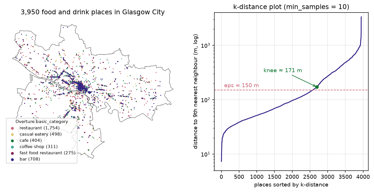
The knee is a guide, not a rule. We rounded down to 150 m because a block in Glasgow’s city-centre grid is about 100–150 m long, so eps = 150 m means “nine other places within about a block”. With NearestNeighbors(n_neighbors=MIN_SAMPLES) on the same points, the first neighbour returned is the point itself, so the last column is the 9th other point. That matches DBSCAN’s definition, in which min_samples includes the point itself.
Step 3: check how sensitive the result is
Before you interpret any cluster, see how much the result depends on the two parameters. The script runs DBSCAN over a grid of eps and min_samples values:
75 100 150 200 300 4005 120 / 29% / 25% 108 / 23% / 28% 99 / 17% / 46% 89 / 13% / 47% 61 / 8% / 59% 48 / 4% / 73%10 49 / 48% / 14% 56 / 37% / 27% 44 / 29% / 31% 37 / 25% / 46% 32 / 16% / 52% 26 / 10% / 71%15 26 / 60% / 14% 20 / 53% / 25% 29 / 38% / 30% 31 / 30% / 35% 25 / 22% / 48% 18 / 15% / 62%20 23 / 70% / 10% 16 / 58% / 25% 19 / 47% / 28% 18 / 38% / 35% 21 / 26% / 47% 18 / 18% / 58%30 9 / 85% / 4% 8 / 73% / 14% 12 / 56% / 27% 9 / 49% / 30% 10 / 36% / 47% 15 / 26% / 50%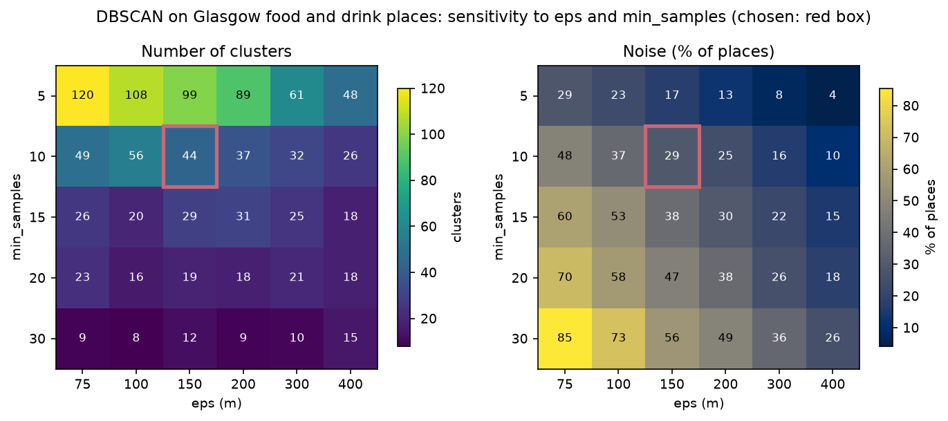
The number of clusters ranges from 120 to 8, and noise from 4% to 85%. Larger eps values do not just grow clusters, they merge them: by eps = 400 m, the largest cluster holds 71% of all places at min_samples 10. Notice also that the number of clusters is not monotonic. At min_samples 15, going from eps 100 m to 200 m first raises the count from 20 to 31, because previously isolated groups pass the density threshold, before merging lowers it again. There is no single right answer here, which is the main motivation for HDBSCAN.
Step 4: HDBSCAN for clusters of different density
DBSCAN uses one density threshold for the whole map: at least 10 places within 150 m, or about 141 places per km². In Glasgow’s centre, places are packed at thousands per km² and are connected to each other almost continuously from the Merchant City to Finnieston, so DBSCAN chains them into one cluster of 1,205 places. In the outer suburbs, a small parade of shops never reaches the threshold and becomes noise.
HDBSCAN (Campello, Moulavi and Sander, 2013) removes eps. It builds the whole hierarchy of DBSCAN solutions across all densities, condenses it into a tree of clusters that persist as the density threshold rises, and keeps the most stable ones. Its main parameter, min_cluster_size, is the smallest group you would call a cluster. scikit-learn has included sklearn.cluster.HDBSCAN since version 1.3; the separate hdbscan package adds plotting tools, soft membership, and a DBCV score.
MIN_CLUSTER = 15hdb = HDBSCAN(min_cluster_size=MIN_CLUSTER, min_samples=MIN_SAMPLES, cluster_selection_method="eom",              copy=True).fit(X_m)hl = hdb.labels_
# the same on latitude/longitudehdb_hav = HDBSCAN(min_cluster_size=MIN_CLUSTER, min_samples=MIN_SAMPLES, metric="haversine").fit(X_rad)
# the hdbscan package gives the condensed tree and a fast DBCV approximationhp = hdbscan.HDBSCAN(min_cluster_size=MIN_CLUSTER, min_samples=MIN_SAMPLES, gen_min_span_tree=True).fit(X_m)sklearn HDBSCAN(min_cluster_size=15, min_samples=10): 54 clusters, noise 28.2%, largest 523 places, median size 34, 63 mssame on lat/lon radians with metric='haversine': 53 clusters, ARI vs metres 0.9772cluster_selection_method='leaf': 67 clusters, noise 34.4%min_cluster_size=10: 88 clusters, noise 34.1%min_cluster_size=25: 39 clusters, noise 22.7%min_cluster_size=50: 18 clusters, noise 29.9%ARI DBSCAN vs HDBSCAN: 0.315HDBSCAN cluster density (places per km2 of convex hull): min 16, median 332, max 3711 (227x range)hdbscan package: 51 clusters, ARI vs sklearn 0.8595, relative_validity_ (fast DBCV approximation) 0.205membership strength: median 0.99; outlier scores > 0.9: 649DBSCAN density floor: 10 places in a 150 m circle = 141 places per km2; 18 of 54 HDBSCAN clusters are sparser than that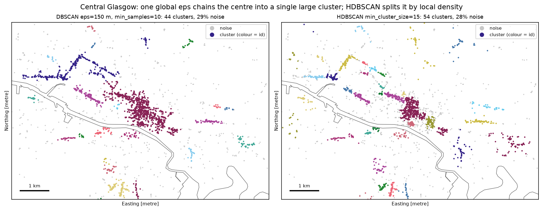
The two clusterings are quite different (ARI 0.315), mostly because HDBSCAN splits DBSCAN’s giant central cluster. HDBSCAN’s largest cluster is the core of the city centre around Buchanan Street, with 523 places.
Three practical notes:
min_samplesandmin_cluster_sizedo different jobs.min_samplessmooths the density estimate (larger values are more conservative and give more noise);min_cluster_sizesets the smallest cluster you care about. If you set onlymin_cluster_size,min_samplesdefaults to the same value.cluster_selection_method: the default"eom"(excess of mass) favours a few large, stable clusters;"leaf"takes the leaves of the tree and gives more, smaller and more uniform clusters (67 here). Usecluster_selection_epsilonif you want HDBSCAN to stop splitting clusters below a set distance.- The two libraries are not identical.
sklearn.cluster.HDBSCANandhdbscan.HDBSCANgave 54 and 51 clusters (ARI 0.86), because of differences in defaults and in how ties are handled. Pick one and report which you used.
Step 5: cluster polygons, profiles and noise
To map clusters as areas or join them to other data, turn each one into a polygon. A convex hull is the smallest convex polygon that contains all the points, and it can include a lot of empty space for elongated clusters. A concave hull follows the points more closely. Shapely 2 has both:
rows = []for c, grp in food[food.hdb >= 0].groupby("hdb"):            # skip the noise label -1    mp = shapely.MultiPoint(grp.geometry.tolist())    convex = shapely.convex_hull(mp)    concave = shapely.concave_hull(mp, ratio=0.3)    top = grp.basic_category.value_counts()    rows.append({"cluster": c, "n": len(grp), "district": grp.district.mode().iloc[0],                 "convex_km2": convex.area / 1e6, "concave_km2": concave.area / 1e6,                 "top": f"{top.index[0].replace('_', ' ')} {top.iloc[0] / len(grp):.0%}",                 "bars": (grp.basic_category == "bar").mean(), "geometry": concave, "convex": convex})hulls = gpd.GeoDataFrame(rows, geometry="geometry", crs=CRS)
nn_noise = BallTree(X_m[hl >= 0]).query(X_m[hl < 0], k=1)[0][:, 0] # distance from noise to nearest cluster54 clusters: convex hulls cover 21.09 km2, concave hulls (ratio 0.3) 9.48 km2 (45% of convex)clustered places: 2,835 of 3,950 (72%) in 5.4% of the city's areaten largest clusters: cluster n district concave_km2 convex_km2 top bars 52 523 G1 0.42 0.54 restaurant 41% 0.29 53 154 G2 0.09 0.09 restaurant 51% 0.26 21 106 G41 0.23 0.40 restaurant 42% 0.11 38 104 G3 0.05 0.08 restaurant 54% 0.14 49 103 G1 0.07 0.10 restaurant 44% 0.32 42 87 G12 0.06 0.13 restaurant 45% 0.15 45 79 G11 0.03 0.07 restaurant 59% 0.16 3 78 G69 1.83 3.22 restaurant 45% 0.23 27 69 G31 0.08 0.18 restaurant 43% 0.12 22 69 G31 0.48 0.84 restaurant 36% 0.20noise: 1,115 places; most common categories: restaurant 42%, bar 17%, casual eatery 12%distance from each noise place to the nearest clustered place: median 297 m, 30% more than 500 m away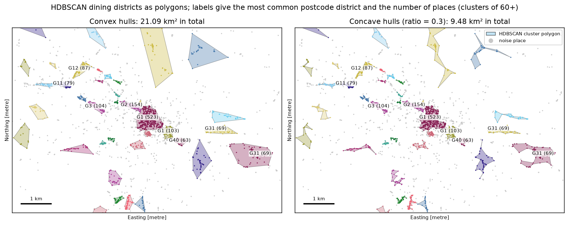
The labels are recognisable. The largest cluster is the core of the city centre around Buchanan Street, split almost evenly between the G1 and G2 postcode districts. Around it are Bath Street and Blythswood (G2), the Trongate end of the Merchant City (G1, 103 places) and Finnieston (G3). Further out are the West End around Byres Road (G12) and Dumbarton Road (G11), Shawlands on the Southside (G41), and two clusters in G31: Duke Street in Dennistoun and the Forge retail park in Parkhead. Clusters that are long and thin, such as a high street, have much smaller concave hulls than convex ones. The G69 cluster in Baillieston, on the city’s eastern edge, has a convex hull of 3.22 km² but only 78 places; it is a loose chain along main roads, and a hull that size is mostly houses and roads.
Noise is a result, not rubbish. 1,115 places (28%) belong to no cluster. Most are ordinary local restaurants, bars and takeaways spread through the residential areas; the median one is about 300 m from the nearest cluster. If you need every point assigned, for example to give every place a “district”, attach noise points to the nearest cluster within a distance you choose, or use hdbscan.approximate_predict with soft membership. Do not just delete them: they are the background against which the clusters stand out.
Step 6: silhouette and DBCV, with caveats
There is no ground truth for “dining districts”, so the only scores available are internal ones that measure how compact and well separated the clusters are.
for name, l in [("DBSCAN", lab), ("HDBSCAN", hl)]:    m = l >= 0    sil = silhouette_score(X_m[m], l[m], random_state=SEED)                      # noise excluded    dbcv = hdbscan.validity.validity_index(X_m.astype(np.float64), l.astype(np.intp))
# null model: the same number of uniformly random points inside the cityU = rng.uniform(lo, hi, size=(len(X_m), 2))U = U[gpd.GeoSeries(gpd.points_from_xy(U[:, 0], U[:, 1]), crs=CRS).within(city).to_numpy()]ul = HDBSCAN(min_cluster_size=MIN_CLUSTER, min_samples=MIN_SAMPLES).fit(U).labels_DBSCAN : silhouette (non-noise only) 0.270 | DBCV -0.022 | 44 clusters | noise 29.1%HDBSCAN : silhouette (non-noise only) 0.516 | DBCV 0.193 | 54 clusters | noise 28.2%null check: 2,380 uniformly random points in the city -> HDBSCAN finds 28 clusters, noise 51%, DBCV 0.096null check: DBSCAN (eps=150 m, min_samples=10) on the same random points -> 0 clusters, noise 100%Read these numbers carefully:
- The silhouette score assumes compact, convex clusters. It compares each point’s average distance to its own cluster with its distance to the nearest other cluster, which penalises long, thin clusters along streets even when they are real. It also has no place for noise, so we computed it on clustered points only. That flatters any method that throws away hard points as noise.
- DBCV (Moulavi and others, 2014) was designed for density-based clusters and does account for noise, but it is slow on large data and sensitive to duplicate points. The
hdbscanpackage’srelative_validity_(0.205 here) is a fast approximation for comparing settings, not the full score. - Algorithms find clusters in random data. HDBSCAN found 28 clusters in uniformly random points and scored a positive DBCV. The real places score higher (0.193 vs 0.096) and DBSCAN’s fixed density threshold rejects the random points entirely, but a positive score does not prove that a cluster is meaningful. Compare against a null model like this one, and check the clusters against local knowledge: here they match well-known restaurant areas.
Step 7: scaling with a BallTree
DBSCAN spends most of its time finding every point’s neighbours within eps. A naive implementation computes all n² distances: for all 41,382 Overture places in Glasgow, a dense distance matrix would need 13.7 GB. A BallTree indexes the points in nested hyperspheres, so each radius query checks only nearby branches. It supports the haversine metric (a KD-tree does not), and scikit-learn’s DBSCAN uses it when you pass algorithm="ball_tree".
allpts = np.radians(g[["lat", "lon"]].to_numpy())                       # every place, not just food and drinktree = BallTree(allpts, metric="haversine")counts = tree.query_radius(allpts, r=EPS / R_EARTH, count_only=True)     # neighbours within 150 m
for algo in ("ball_tree", "brute"):    DBSCAN(eps=EPS / R_EARTH, min_samples=MIN_SAMPLES, metric="haversine", algorithm=algo).fit(Xs)HDBSCAN(min_cluster_size=MIN_CLUSTER, min_samples=MIN_SAMPLES, metric="haversine").fit(Xs)
HDBSCAN(min_cluster_size=MIN_CLUSTER, min_samples=MIN_SAMPLES).fit(np.column_stack([g.geometry.x, g.geometry.y])) # projectedall Overture places in Glasgow City: 41,382BallTree build 15 ms; 41,382 radius queries of 150 m in 451 ms; neighbours per point median 71, max 1,301a dense haversine distance matrix for all of them would need 13.7 GBn= 2,000: DBSCAN ball_tree 0.01 s | brute 0.02 s | HDBSCAN 0.11 sn= 4,000: DBSCAN ball_tree 0.03 s | brute 0.04 s | HDBSCAN 0.38 sn= 8,000: DBSCAN ball_tree 0.07 s | brute 0.16 s | HDBSCAN 1.33 sn=16,000: DBSCAN ball_tree 0.19 s | brute 0.61 s | HDBSCAN 5.20 sn=32,000: DBSCAN ball_tree 0.44 s | HDBSCAN 20.16 sn=41,382: DBSCAN ball_tree 0.70 s | HDBSCAN 34.05 sHDBSCAN on all 41,382 places in projected metres (KD-tree): 6.10 s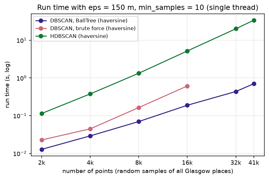
DBSCAN with a BallTree clustered all 41,382 places in well under a second. Brute force was already 3.2 times slower at 16,000 points and its memory use grows with n². Two things matter more than the algorithm, though:
- DBSCAN’s cost depends on how many neighbours each point has. In the densest part of Glasgow, one place has 1,301 others within 150 m. A large eps on dense data makes every query return thousands of points, and run time and memory rise sharply. Keep eps as small as the problem allows.
- HDBSCAN is much slower with haversine. Its fast algorithms (Prim’s algorithm on a KD-tree, or Borůvka) need a metric a KD-tree supports. With haversine it falls back to a BallTree and took 34 s for 41,382 points. On the same places in projected metres it uses a KD-tree and took 6.1 s, more than five times faster, which is another reason to prefer projected coordinates for a city.
For millions of points (a national GPS trace archive, for example), split the data by region with a buffer, aggregate to a grid first such as H3 hexagons, or use a GPU implementation such as RAPIDS cuML.
Limitations and honest caveats
- Overture places are not a census of businesses. They come from several sources, including Meta and Microsoft, with varying completeness and some duplicates and closed businesses. The confidence filter removes some of these but not all, and categories are assigned by a model. Treat counts as indicative.
- Clusters depend on what you include. Adding takeaways, pubs or hotels, or using a different confidence threshold, would change the clusters. The six categories here are a choice, not a definition of a “dining district”.
- The parameters are choices too. The k-distance knee,
min_samples,min_cluster_sizeand the hull ratio all change the result. Show a sensitivity check like Step 3 and report the values you used. - Point density is not activity. A cluster of many small cafés and a single large restaurant have very different numbers of customers. For footfall or spending, use other data.
- Edge effects. Places just outside Glasgow City, in East Dunbartonshire or Renfrewshire for example, are ignored, so clusters on the boundary are truncated. Buffer the study area if that matters.
- Internal scores are not validation (Step 6). They compare settings on the same data; they do not prove that a cluster is real.
Frequently asked questions
How do I use DBSCAN with latitude and longitude in Python?
Convert to radians in [lat, lon] order and pass metric="haversine": DBSCAN(eps=150 / 6_371_008.8, min_samples=10, metric="haversine", algorithm="ball_tree").fit(np.radians(df[["lat", "lon"]])). The eps is in radians, so divide your distance in metres by the Earth’s radius. Alternatively, reproject to a local metric CRS with GeoPandas and use eps in metres with the default metric; for a city the results are practically identical.
How do I choose eps for DBSCAN?
Pick min_samples first, then compute each point’s distance to its (min_samples − 1)th nearest other point with NearestNeighbors, sort the distances and plot them. Choose eps near the knee, where the curve turns sharply upwards, and round it to a value that makes sense on the ground. Then run a small sensitivity grid around it, because the knee is often a range rather than a point.
What is the difference between DBSCAN and HDBSCAN?
DBSCAN uses one density threshold, set by eps and min_samples, for the whole dataset. HDBSCAN considers all thresholds, keeps the clusters that persist longest, and so can find dense and sparse clusters in the same data. HDBSCAN is usually the better default for real geographic points, whose density varies across a city. DBSCAN is simpler to explain (“at least 10 places within 150 m”) and faster, which can matter for reporting or very large data.
How do I turn DBSCAN clusters into polygons?
Group the points by label, skip label −1 (noise), and build a hull for each group: shapely.convex_hull(shapely.MultiPoint(points)) or shapely.concave_hull(..., ratio=0.3). Concave hulls follow elongated clusters more closely; lower ratios give tighter shapes. For smoother areas, buffer the points by eps/2 and dissolve them.
Should I report the silhouette score for DBSCAN?
Only with caveats. The silhouette assumes compact, convex clusters and has no place for noise, so it is computed on the clustered points only and can reward throwing hard points away as noise. DBCV is designed for density-based clustering and is a better choice, but both are internal measures: use them to compare settings on the same data, and test your clusters against random points and local knowledge.
Can I use DBSCAN for GPS trajectories and stop detection?
Yes. Clustering the GPS fixes of one device with a small eps (for example 50 m) and a min_samples that corresponds to a few minutes of fixes finds places where the device stayed. For proper stay-point detection, also use time: split the trace into time windows first, or use a dedicated library such as scikit-mobility or MovingPandas.
Next steps
- For areas rather than points, cluster census Output Areas by their population characteristics in our companion tutorial, geodemographic classification in Python, which uses k-means and contiguous regionalisation with spopt.
- Test whether points or counts are significantly clustered, rather than describing clusters, with hot spot analysis in Python (Getis-Ord Gi*).
- Read Overture data for any city and query it with SQL in GeoParquet and DuckDB with Overture Maps.
- Aggregate points to a hexagon grid instead of clustering them with H3 hexagon grids in Python.
- Measure walking distances between clusters along streets rather than as the crow flies with OSMnx street network analysis.
- Join the cluster polygons to other data, such as census areas, with spatial joins in GeoPandas. The script writes
output/glasgow_dining_clusters.gpkgwith the places and the concave hulls.
Data and licences
- Places: Overture Maps Foundation, Places theme, release 2026-10-21.0, read from
s3://overturemaps-us-west-2/on 27 October 2026. Licensed under the Community Data License Agreement – Permissive 2.0; some sources carry their own attribution requirements, listed in the Overture attribution guide. - Boundary: Office for National Statistics, Local Authority Districts (May 2026) Boundaries UK BGC, from the Open Geography Portal. Source: Office for National Statistics licensed under the Open Government Licence v3.0. Contains OS data © Crown copyright and database right 2026.
- Further reading: Ester, M., Kriegel, H.-P., Sander, J. and Xu, X. (1996), “A density-based algorithm for discovering clusters in large spatial databases with noise”, Proceedings of KDD-96: 226–231; Campello, R. J. G. B., Moulavi, D. and Sander, J. (2013), “Density-based clustering based on hierarchical density estimates”, PAKDD 2013: 160–172; Moulavi, D. and others (2014), “Density-based clustering validation”, SIAM International Conference on Data Mining: 839–847; McInnes, L., Healy, J. and Astels, S. (2017), “hdbscan: Hierarchical density based clustering”, Journal of Open Source Software 2(11): 205.
- Code:
dbscan_dining_districts.py, tested with Python 3.12.0, scikit-learn 1.9.1, hdbscan 0.8.44, geopandas 1.2.0, shapely 2.2.0, pyogrio 0.13.0, pyproj 3.8.0, numpy 2.5.4, pandas 3.1.0, scipy 1.18.1, matplotlib 3.11.2, duckdb 1.5.6, pyarrow 26.0.0 and requests 2.34.2.
Key terms
- DBSCAN
- Density-Based Spatial Clustering of Applications with Noise. A point with at least min_samples points within distance eps is a core point; clusters are chains of core points and their neighbours, and everything else is noise.
- HDBSCAN
- Hierarchical DBSCAN. It runs DBSCAN at every possible eps at once, builds a tree of clusters as the density threshold rises, and keeps the most persistent ones, so clusters of different densities can coexist.
- Haversine distance
- The great-circle distance between two points on a sphere, computed from their latitude and longitude. scikit-learn's version takes [lat, lon] in radians and returns radians, so multiply by the Earth's radius to get metres.
- k-distance plot
- Every point's distance to its k-th nearest neighbour, sorted in ascending order. The knee of the curve, where distances start to rise sharply, suggests a value for eps.
- Core, border and noise points
- A core point has at least min_samples neighbours within eps (counting itself). A border point is within eps of a core point but is not core itself. Noise points are neither and get the label -1.
- Concave hull
- A polygon that wraps a set of points more tightly than the convex hull by allowing inward bends. In Shapely the ratio parameter runs from 0 (tightest) to 1 (the convex hull).
- DBCV
- Density-Based Clustering Validation, an internal score from -1 to 1 designed for density-based clusters of any shape. It compares the sparsest region inside each cluster with the densest gap between clusters.
- BallTree
- A spatial index that nests points in hyperspheres, so radius and nearest-neighbour queries need to check only a fraction of the points. Unlike a KD-tree, it supports the haversine metric.
Data for this tutorial
- Overture Maps · The places theme: tens of millions of points of interest worldwide as GeoParquet on Amazon S3 and Azure
- OpenStreetMap · An alternative source of restaurants, cafés and pubs (amenity tags) for the same workflow
- Open Geography Portal · ONS Local Authority Districts (May 2026) boundary for Glasgow City
Licences and formats for each source are listed in the GIS data sources catalogue.