Point pattern analysis in Python: quadrats, nearest neighbour and Ripley's K on Camden's street trees

Short answer: point pattern analysis in Python tests whether a set of point locations is clustered, random or regular. Compare the pattern with complete spatial randomness (CSR) in a clearly defined study window. Use a quadrat chi-squared test or the Clark-Evans nearest-neighbour index for a single overall answer. Then use Ripley’s K (or L) function, with Monte Carlo simulation envelopes from pointpats.random.poisson, to see at which distances the clustering happens. Correct for edge effects, and finish with a global test such as the MAD test, because an envelope checked at many distances is not a single test. For Camden’s 3,292 London plane trees, every test rejects CSR: the Clark-Evans ratio is 0.38, and L(r) − r peaks at about 103 m around r = 200 m, far outside a CSR envelope of ±3 m.

This is Part 1 of a two-part series. It tests whether and at what scale points cluster. Part 2, kernel density estimation in Python, turns the same trees into a density surface (a “heatmap”). It covers bandwidth selection, a GeoTIFF export, and a case-control relative-risk map.

You will learn how to:

1. choose a study window and see why it matters;
2. run a quadrat count with a chi-squared test that handles clipped cells;
3. compute the Clark-Evans index with and without the Donnelly edge correction, and check it by simulation;
4. estimate G, F, K and L functions with border correction and CSR envelopes;
5. measure how much the window shape and edge correction change K;
6. replace pointwise envelopes with a global MAD test, and test against a better null: random labelling.

All outputs below are real results from point_pattern_analysis.py, run on 27 October 2026 with Python 3.12.0, pointpats 2.6.0, geopandas 1.2.0, shapely 2.2.0, scipy 1.18.1 and numpy 2.5.4. The script takes about a minute.

The data: Camden’s council trees

The London Borough of Camden publishes Trees In Camden: every tree the council manages on streets, housing estates, parks and school grounds, with its species, height, crown spread and British National Grid coordinates. It is open data under the Open Government Licence and is updated daily. We study one species, the London plane (Platanus × hispanica), the classic London street tree. The study window is the borough boundary from the ONS Open Geography Portal.

TREES_URL = "https://opendata.camden.gov.uk/api/views/csqp-kdss/rows.csv?accessType=DOWNLOAD"
CRS = "EPSG:27700"    # British National Grid, metres

df = pd.read_csv(download(TREES_URL, DATA / "trees_in_camden.csv"), low_memory=False)
df = df[df.Easting > 0]
trees = gpd.GeoDataFrame(df, geometry=gpd.points_from_xy(df.Easting, df.Northing), crs=CRS)

boundary = gpd.read_file(download(LAD_URL, DATA / "camden_lad.geojson", where=f"LAD26CD='{LAD}'",
                                  outFields="LAD26CD,LAD26NM", outSR=27700, f="geojson")).set_crs(CRS, allow_override=True)
W = boundary.geometry.iloc[0]
trees = trees[shapely.contains_xy(W, trees.Easting, trees.Northing)]

planes = trees[trees["Common Name"] == SPECIES]
planes = planes.drop_duplicates(["Easting", "Northing"])
xy = np.column_stack([planes.Easting, planes.Northing]).astype(float)
n = len(xy)

df.Easting > 0 drops the few records with no coordinates. SPECIES is "London plane" and LAD is Camden’s code, "E09000007".

Point pattern statistics assume that no two points share a location, so we drop exact duplicates; there was one.

28,128 tree records (snapshot uploaded 26 October 2026)
27,883 with coordinates
27,604 inside the borough boundary (21.78 km2, perimeter 26.2 km)
by contract area: {'Highways': 11928, 'Housing': 9805, 'Parks': 4308, 'Education': 1347, 'Corporate Landlord': 193, 'Valuers': 23}
London plane: 3,293 records, 1 at duplicate coordinates dropped -> n = 3,292
  by contract area: {'Highways': 1987, 'Housing': 697, 'Parks': 541, 'Education': 63, 'Corporate Landlord': 4}
all council trees at distinct locations: 27,403
windows: borough 21.78 km2 | within 100 m of a council tree 17.77 km2 | bounding box of the planes 47.31 km2
intensity: 1.51 planes per hectare (151 per km2)

Step 1: choose the study window

The window is the area where a point could have occurred. It sets the intensity λ (points per unit area), and with it every expected value under CSR. It is the most consequential choice in a point pattern analysis, and the one most often made by accident. The script builds three windows:

• the borough boundary (21.8 km²), the obvious administrative choice;
• a support window: the parts of Camden within 100 m of any council tree (17.8 km²). It removes Hampstead Heath, the Regent’s Park edge and other land where the council does not plant trees;
• the bounding box of the planes (47.3 km²). Several libraries use it by default, and it is more than twice the size of the borough.

all_xy = np.unique(np.column_stack([trees.Easting, trees.Northing]).astype(float), axis=0)
support = shapely.intersection(W, shapely.union_all(shapely.buffer(shapely.points(all_xy), 100, quad_segs=4)))
bbox_area = np.ptp(xy[:, 0]) * np.ptp(xy[:, 1])
lam = n / W.area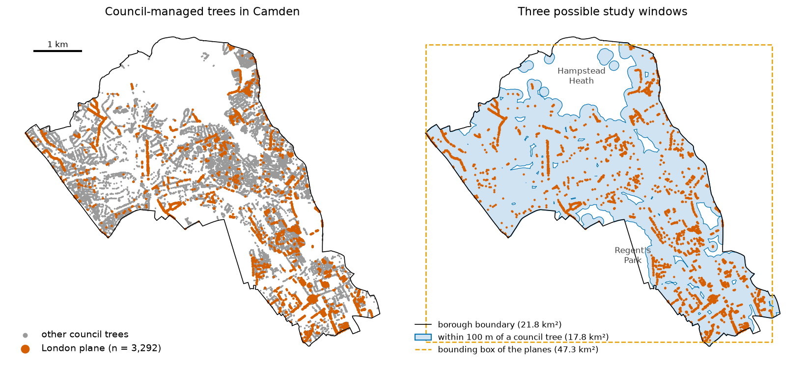

We use the borough as the main window, and return to the other two in Step 5.

Step 2: quadrat counts and a chi-squared test

The oldest test cuts the window into cells (quadrats), counts the points in each, and compares the counts with CSR using a chi-squared test. Under CSR, each cell’s expected count is proportional to its area. Most quadrat tools, including pointpats.QStatistic, give every cell the same expected count. That is wrong for cells cut by an irregular boundary, so we clip 500 m squares to the borough and weight the expected counts by area:

def quadrats(size):
    """Square cells clipped to the borough; slivers under a quarter of a full cell are dropped."""
    cells = [shapely.box(x, y, x + size, y + size) for x in np.arange(xmin, xmax, size) for y in np.arange(ymin, ymax, size)]
    g = gpd.GeoDataFrame(geometry=gpd.GeoSeries(cells, crs=CRS).intersection(W), crs=CRS)
    return g[g.area >= 0.25 * size * size].reset_index(drop=True)


def quadrat_test(grid):
    grid["count"] = gpd.sjoin(pts, grid, predicate="within").groupby("index_right").size().reindex(grid.index, fill_value=0)
    grid["expected"] = grid["count"].sum() / grid.area.sum() * grid.area   # proportional to each clipped cell's area
    chi2 = (((grid["count"] - grid["expected"]) ** 2) / grid["expected"]).sum()
    return chi2, len(grid) - 1, stats.chi2.sf(chi2, len(grid) - 1)

98 cells (60 complete squares), 3,258 planes counted, 10 empty cells
chi2 = 2,770.6, df = 97, p < 1e-300
variance/mean ratio on complete squares: 28.12 (1 under CSR, > 1 clustered, < 1 regular)
   250 m squares: 368 cells, chi2 = 5,399.4, df = 367, p < 1e-300
  1000 m squares: 28 cells, chi2 = 1,487.4, df = 27, p = 4.9e-297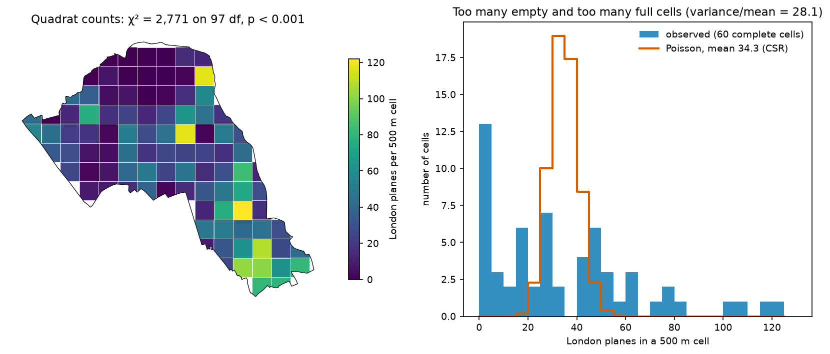

The verdict is unambiguous: the variance of the counts is 28 times their mean, while CSR gives a ratio of 1. A ratio above 1 means clustering. The test does not depend on the cell size here, but the χ² statistic does: it is 1,487 with 1 km squares and 5,399 with 250 m squares. Quadrat tests are a form of the modifiable areal unit problem (MAUP), the same issue the hot spot analysis tutorial explores with hexagons. Two further caveats apply. The cells must have enough expected points (5 is the usual minimum), and the test says nothing about the scale of the clustering.

Step 3: the Clark-Evans nearest-neighbour index

The average nearest-neighbour test, also called the Clark-Evans test, compares the mean distance from each point to its nearest neighbour with the value expected under CSR, 0.5/√λ. The ratio R is below 1 for clustered patterns and above 1 for regular ones. The textbook formula ignores the boundary. Points near the edge have their true nearest neighbour outside the window, so their observed distances are too long. Donnelly’s (1978) correction adds a perimeter term:

nnd = cKDTree(xy).query(xy, k=2)[0][:, 1]
A, P = W.area, W.length
exp_naive = 0.5 / np.sqrt(n / A)
se_naive = 0.26136 / np.sqrt(n * n / A)
R = nnd.mean() / exp_naive
z = (nnd.mean() - exp_naive) / se_naive
# Donnelly (1978): expected NND and its standard error corrected for the window's perimeter
exp_don = 0.5 * np.sqrt(A / n) + (0.0514 + 0.041 / np.sqrt(n)) * P / n
se_don = np.sqrt(0.0703 * A / n ** 2 + 0.037 * P * np.sqrt(A / n ** 5))

# CSR in the borough window with pointpats: NSIM patterns of n points each
sims = pp_random.poisson(W, size=(n, NSIM), rng=SEED)
sim_mean_nnd = np.array([cKDTree(s).query(s, k=2)[0][:, 1].mean() for s in sims])
p_ce = (1 + (sim_mean_nnd <= nnd.mean()).sum()) / (NSIM + 1)

pointpats.random.poisson accepts a shapely polygon. With size=(n, NSIM) it returns an array of 199 patterns, each with n points, in one call. We reuse these patterns for every envelope below.

mean NND 15.5 m, median 10.4 m, 10.5% under 5 m, 74.5% under 15 m
CSR expectation 0.5/sqrt(lambda) = 40.7 m -> R = 0.380, z = -68.0, p < 1e-300
Donnelly edge-corrected expectation 41.1 m -> R = 0.376, z = -66.5
Monte Carlo: mean NND under CSR in the borough 41.1 m (range 40.3-42.1); one-sided p = 0.005 (floor 0.005)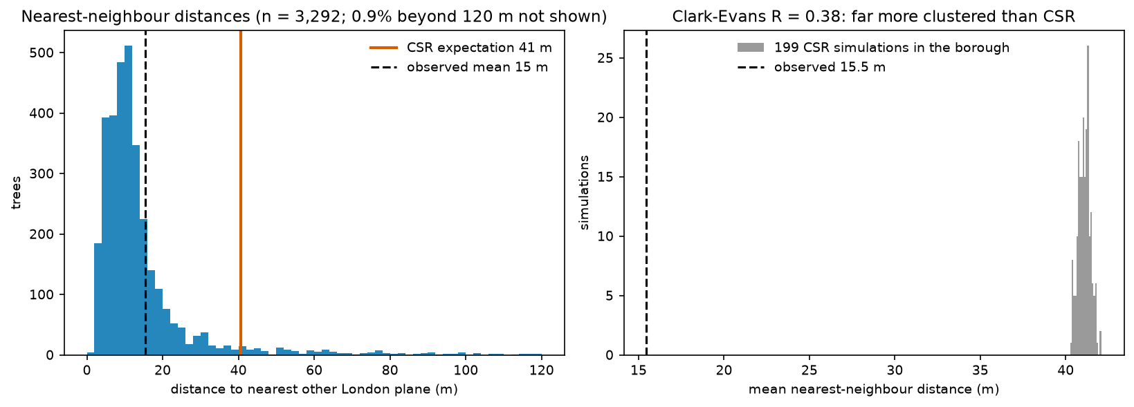

R = 0.38 means the planes are much closer together than random trees would be. The simulated mean (41.1 m) matches Donnelly’s corrected value exactly, which confirms the correction. With n = 3,292 the uncorrected formula is only 1% off, but for small samples in irregular windows the difference matters. The simulation p-value is 0.005, which is simply 1/(199 + 1): the smallest value 199 simulations can give. It does not mean the evidence is “only” p = 0.005.

Step 4: G, F, K and L functions with CSR envelopes

Single-number tests hide the scale of clustering. The second-order summary functions show how the pattern departs from CSR as distance r grows:

• G(r): the share of points whose nearest neighbour is within r. Clustering pushes G above CSR.
• F(r): the share of random locations within r of a point (the empty-space function). Clustering leaves big gaps, so F falls below CSR.
• K(r): the mean number of further points within r of a point, divided by λ. Under CSR K(r) = πr². L(r) − r = √(K/π) − r is 0 under CSR and easier to read.

pointpats has g, f, k and l functions and simulation-based tests, but in version 2.6.0 they have limits for this job. They estimate λ from the bounding box of the points, not from your window. Their CSR simulations are drawn in the bounding box. And they do not yet implement edge correction (the edge_correction argument raises NotImplementedError). So we write the border-corrected (reduced-sample) estimators ourselves with scipy.spatial.cKDTree, in about 30 lines, and use pointpats for the simulations:

def ratio_border(values, b, r):
    """Border-corrected (reduced-sample) estimate of P(value <= r) using only points at least r from the edge:
    #{value <= r <= b} / #{b >= r}."""
    ok = values <= b
    num = np.searchsorted(np.sort(values[ok]), r, "right") - np.searchsorted(np.sort(b[ok]), r, "left")
    den = len(b) - np.searchsorted(np.sort(b), r, "left")
    return num / np.maximum(den, 1)


def g_func(pts, b, r):
    return ratio_border(cKDTree(pts).query(pts, k=2)[0][:, 1], b, r)


def f_func(pts, grid_pts, grid_b, r):
    return ratio_border(cKDTree(pts).query(grid_pts, k=1)[0], grid_b, r)


def k_func(pts, b, r, area, correct=True):
    """Ripley's K. correct=True: border correction, so each point counts only at distances it can 'see' in full."""
    pairs = cKDTree(pts).query_pairs(r.max(), output_type="ndarray")
    d = np.hypot(*(pts[pairs[:, 0]] - pts[pairs[:, 1]]).T)
    lam_hat = len(pts) / area
    if not correct:
        return 2 * np.searchsorted(np.sort(d), r, "right") / (len(pts) * lam_hat)
    i = np.concatenate([pairs[:, 0], pairs[:, 1]]); dd = np.concatenate([d, d])
    bi = b[i]; ok = dd <= bi
    num = np.searchsorted(np.sort(dd[ok]), r, "right") - np.searchsorted(np.sort(bi[ok]), r, "left")
    m = len(b) - np.searchsorted(np.sort(b), r, "left")
    return num / (np.maximum(m, 1) * lam_hat)


def l_minus_r(K, r):
    return np.sqrt(K / np.pi) - r


def edge_dist(pts, window):
    return shapely.distance(shapely.points(pts), window.boundary)

b is each point’s distance to the window boundary. At distance r, only points with b ≥ r contribute, because their whole disc of radius r lies inside the window. That is the border correction. It is unbiased but wastes data at large r. At 500 m, only 1,398 of the 3,292 planes are far enough from Camden’s long, thin boundary. The F function uses a 20 m grid of 54,441 sample locations inside the borough. Then we run the same functions on all 199 CSR patterns and take the minimum and maximum at each r as the envelope:

r_g = np.arange(0, 81, 1.0)
r_f = np.arange(0, 401, 5.0)
r_k = np.arange(0, 501, 5.0)
b_obs = edge_dist(xy, W)
obs = {"G": g_func(xy, b_obs, r_g), "F": f_func(xy, gpts, gb, r_f), "K": k_func(xy, b_obs, r_k, A)}
sim = {"G": [], "F": [], "K": [], "K_raw": []}
for s in sims:
    bs = edge_dist(s, W)
    sim["G"].append(g_func(s, bs, r_g)); sim["F"].append(f_func(s, gpts, gb, r_f))
    sim["K"].append(k_func(s, bs, r_k, A)); sim["K_raw"].append(k_func(s, bs, r_k, A, correct=False))
sim = {key: np.array(v) for key, v in sim.items()}
L_obs, L_sim = l_minus_r(obs["K"], r_k), l_minus_r(sim["K"], r_k)

54,441 F-function sample points on a 20 m grid; 1,398 of 3,292 planes are at least 500 m from the boundary
G: above the envelope at 3-80 m (78 of 81 distances), below at none
F: above the envelope at none (0 of 81 distances), below at 10-400 m
K: above the envelope at 5-500 m (100 of 101 distances), below at none
  r =  10 m: L(r) - r =   31.6 m (CSR envelope  -1.6 to   1.8)
  r =  50 m: L(r) - r =   78.6 m (CSR envelope  -1.5 to   1.5)
  r = 100 m: L(r) - r =   95.3 m (CSR envelope  -1.8 to   1.9)
  r = 200 m: L(r) - r =  103.4 m (CSR envelope  -3.0 to   3.0)
  r = 400 m: L(r) - r =   89.0 m (CSR envelope  -6.6 to   7.2)
G(15 m) = 0.76 (CSR envelope 0.083-0.119)
F(100 m) = 0.55 (CSR envelope 0.99-1.00)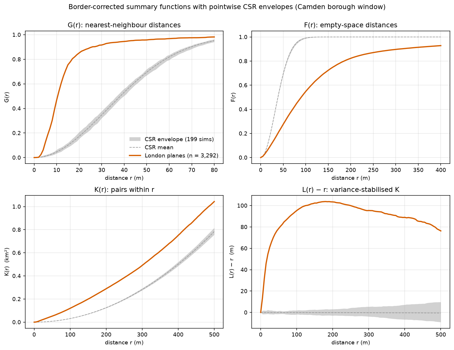

How to read this:

• G: 76% of planes have another plane within 15 m. Under CSR, only 8–12% would. This is the short-range spacing of avenues.
• F: from a random spot in Camden, only 55% of locations have a plane within 100 m. Under CSR, essentially all of them would. Large parts of the borough have no planes at all.
• L(r) − r rises steeply to about 80 m by r = 50 m, then flattens near 100 m between 100 and 300 m. Within a radius r, a typical plane has as many neighbours as a random tree would have within a radius of r + 100 m. Do not read the peak as “the cluster size”. L − r keeps rising while a bigger radius still adds neighbours from the same avenues and estates, then levels off once the radius passes the scale of those groups. Read the shape of the curve, not one maximum.

Step 5: the window and the edge correction change the answer

The next step compares four versions of the L function for the same 3,292 trees. They use pointpats.l with its default bounding-box area, the borough with and without border correction, and the support window that excludes land without council trees:

_, l_pp = pointpats.l(xy, support=r_k, linearized=True)       # pointpats: bounding-box area, no edge correction
L_raw = l_minus_r(k_func(xy, b_obs, r_k, A, correct=False), r_k)
b_sup = edge_dist(xy, support)
L_sup = l_minus_r(k_func(xy, b_sup, r_k, support.area), r_k)
m_sup = np.array([(b_sup >= rr).sum() for rr in r_k])
L_sup[m_sup < 100] = np.nan   # too few planes far enough from the holes in this window to estimate K
L_raw_sim = l_minus_r(sim["K_raw"], r_k)

planes at least r from the window edge: borough 2,210 at 250 m, 1,398 at 500 m | support window 898 at 250 m, 27 at 500 m (curve dropped beyond 445 m)
r = 100 m: L - r =  184.7 (pointpats, bounding box) |   93.2 (borough, no correction) |   95.3 (borough, border) |   78.7 (100 m support window, border)
           CSR mean in the borough:   -1.3 without correction,  -0.1 with border correction
r = 250 m: L - r =  263.3 (pointpats, bounding box) |   98.3 (borough, no correction) |   99.9 (borough, border) |   77.2 (100 m support window, border)
           CSR mean in the borough:   -7.5 without correction,  -0.2 with border correction
r = 500 m: L - r =  333.0 (pointpats, bounding box) |   65.1 (borough, no correction) |   76.3 (borough, border) |    nan (100 m support window, border)
           CSR mean in the borough:  -28.9 without correction,  -0.5 with border correction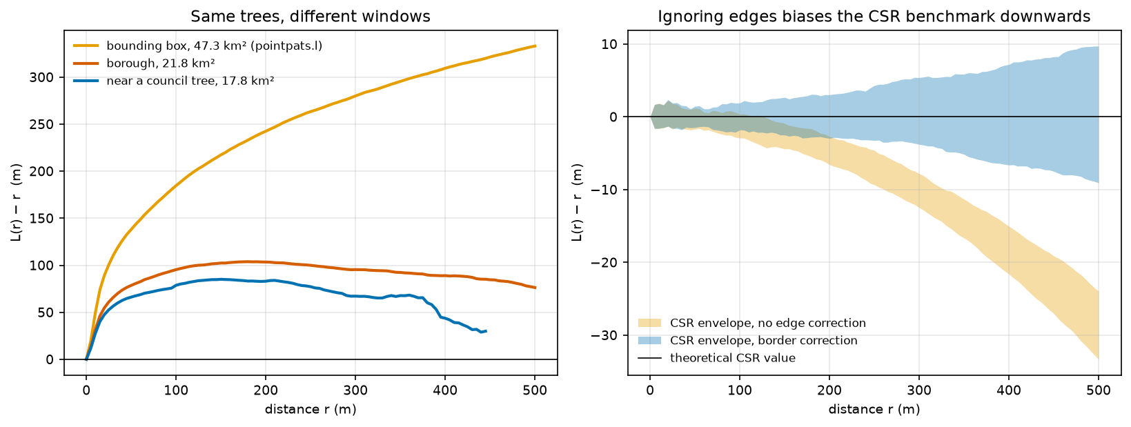

Three lessons:

1. The bounding box exaggerates clustering. pointpats divides by the 47.3 km² box, so λ is too small, and “more neighbours than expected” is partly “the box is mostly outside Camden”. Always pass, or compute with, the real window.
2. Without edge correction, the CSR benchmark drifts. For random patterns in Camden, uncorrected L − r averages −29 m at 500 m, because points near the boundary lose neighbours outside it. The observed curve is biased in the same way (65 m instead of 76 m). An uncorrected curve compared with uncorrected simulations in the same window is still a fair test. The magnitude is wrong, though, and comparing it with the theoretical zero line is not fair.
3. A tighter window gives weaker clustering, and that is a different question. In the support window, L − r is about 78 m instead of 95 m at 100 m. Excluding Hampstead Heath removes part of the “clustering”, which was really “no trees on the Heath”. Which window is right depends on what you are asking. The border method also runs out of data in a window full of holes: only 27 planes are 500 m from the support window’s edge. Translation or isotropic (Ripley) corrections use more of the data; R’s spatstat implements them if you need them.

Step 6: a global test, and a better null hypothesis

Why the envelope is not a test across all distances

With 199 simulations, a pointwise min–max envelope has a 1% chance (2/200) of being exceeded at a single, pre-chosen distance. But we looked at 101 distances. The script checks how often a pattern that really is CSR leaves the envelope of the other 198 anywhere between 0 and 500 m:

MAD on L(r) - r, 0-500 m: observed 103.9 m; CSR simulations 2.5 m median, 10.3 m max; p = 0.005
pointwise envelope check: 13% of CSR patterns leave the envelope of the other 198 at one or more of 101 distances

So “the curve leaves the envelope somewhere” has a false-positive rate of about 13%, not 1%. This is the multiple-testing problem in another form. The fix is a global test that reduces each curve to one number. The maximum absolute deviation (MAD) test (Diggle 1986; Loosmore and Ford 2006) uses the largest gap between a curve and the mean of the simulations, over the whole range of r:

def mad_test(obs_curve, sim_curves):
    """Maximum absolute deviation test (Diggle 1986; Loosmore and Ford 2006) over all distances at once."""
    t_obs = np.abs(obs_curve - sim_curves.mean(axis=0)).max()
    # each simulation is compared with the mean of the others, so it is treated exactly like the data
    total = sim_curves.sum(axis=0)
    t_sim = np.array([np.abs(s - (total - s) / (len(sim_curves) - 1)).max() for s in sim_curves])
    return t_obs, t_sim, (1 + (t_sim >= t_obs).sum()) / (len(t_sim) + 1)

The planes’ MAD is 104 m, while no CSR simulation exceeds 10.3 m. Choose the range of r before looking at the data. The test is valid for the range you fix in advance, and shopping for the range brings the multiple-testing problem back. Global envelopes with an exact overall level (Myllymäki et al. 2017) are available in R’s GET package. They give both a single p-value and a graphical band.

Random labelling: are planes more clustered than trees in general?

Rejecting CSR here was never in doubt. Street trees can only grow along streets, in estates and in parks, so any species would be clustered relative to a uniform scatter over the borough. A more useful question is whether London planes are more clustered than council trees in general. Random labelling answers it. Draw 3,292 locations at random from all 27,403 council-tree locations, compute L − r, repeat 199 times, and compare. This null keeps the inhomogeneous pattern of where trees can be, and asks only whether the plane labels are spread at random among those locations.

rng = np.random.default_rng(SEED)
b_all = edge_dist(all_xy, W)
L_rl = []
for _ in range(NSIM):
    idx = rng.choice(len(all_xy), size=n, replace=False)
    L_rl.append(l_minus_r(k_func(all_xy[idx], b_all[idx], r_k, A), r_k))
L_rl = np.array(L_rl)
t_obs_rl, t_sim_rl, p_mad_rl = mad_test(L_obs, L_rl)

L - r vs random labelling: above the envelope at 5-465 m (93 of 101 distances), below at none
  r =  20 m: planes   54.7 m | all council trees   20.1 m | random-label envelope   18.3 to   22.2
  r =  50 m: planes   78.6 m | all council trees   31.0 m | random-label envelope   28.8 to   34.8
  r = 100 m: planes   95.3 m | all council trees   42.0 m | random-label envelope   38.7 to   46.8
  r = 200 m: planes  103.4 m | all council trees   52.9 m | random-label envelope   47.6 to   58.7
  r = 400 m: planes   89.0 m | all council trees   66.4 m | random-label envelope   56.5 to   75.9
MAD test vs random labelling: observed 54.4 m; simulations median 4.6 m, max 14.9 m; p = 0.005
  restricted to 0-100 m: p = 0.005
  restricted to 100-500 m: p = 0.005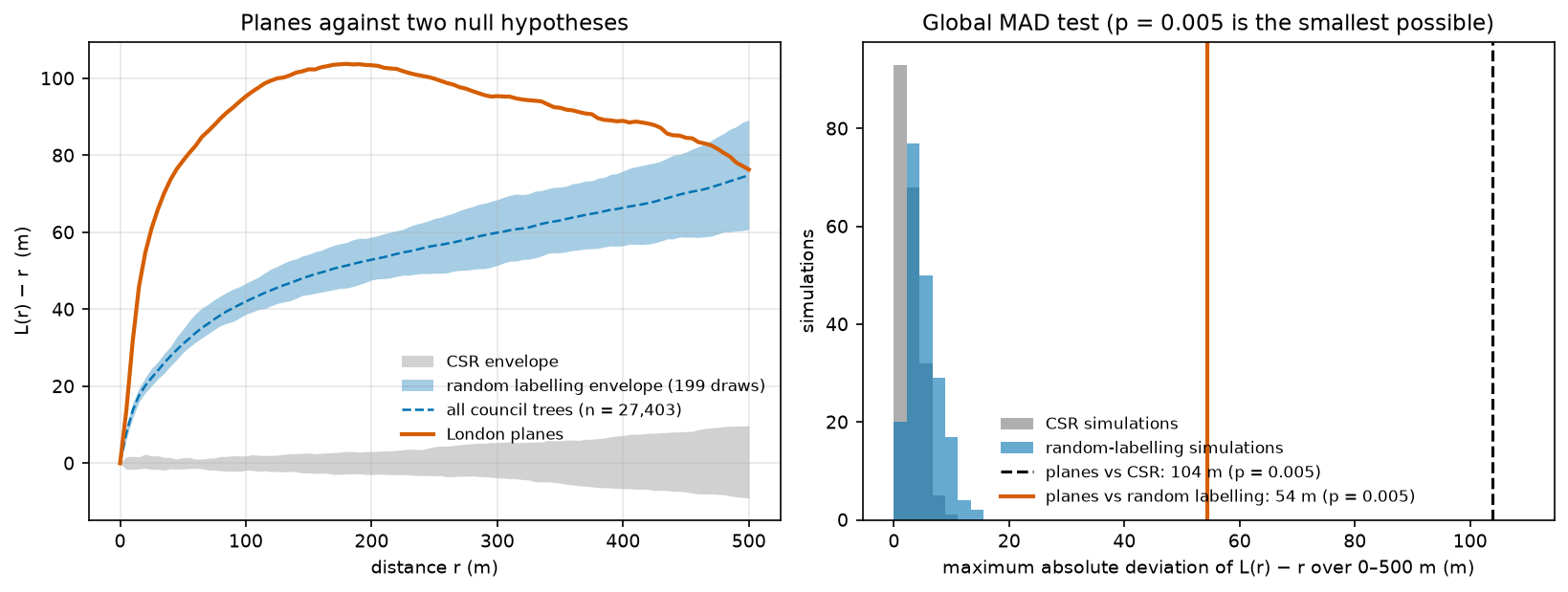

About half of the planes’ apparent clustering against CSR is just “trees grow where streets are”. The rest is real at the species level: L − r for planes is 55 m at 20 m, against 18–22 m for random sets of council trees. Planes are planted as avenues and estate groups of one species, and the global test confirms that this is not chance (p = 0.005). The curves meet at about 465 m, so beyond a few hundred metres planes are spread like council trees in general.

The script saves the cleaned planes and both windows as output/camden_london_planes.gpkg and output/camden_windows.gpkg for use in QGIS.

Limitations and honest caveats

• This is the council’s inventory, not every tree. Trees in private gardens, Royal Parks (Regent’s Park and Primrose Hill) and the City of London’s Hampstead Heath are not in it. The pattern describes council planting and management, not the urban forest. The data are updated daily, so counts will change slightly if you rerun the script.
• CSR is a straw man for street trees. Rejecting it is almost guaranteed. Random labelling is the more informative test here, but it assumes every council-tree location could equally have held a plane. It ignores, for example, that planes need wide pavements.
• Clustering is not a process. Second-order functions describe how points are arranged, not why. A cluster process (Thomas, Matérn) and an inhomogeneous Poisson process can give identical K functions. Separating them needs covariates and models, such as Poisson point process regression (spatstat in R).
• Border correction discards data. It is unbiased but noisy at large r, and in windows with holes it fails sooner (Step 5). Do not interpret K beyond about a quarter of the window’s short side.
• Envelopes are not confidence intervals. They show the range of the null model, not the uncertainty of the observed curve. Choose the distance range for a global test in advance.
• Duplicates and precision. The coordinates are recorded to the metre, and one exact duplicate was removed. Distances below a metre or two are not meaningful.

Frequently asked questions

How do I calculate Ripley’s K in Python?

pointpats.k(xy, support=distances) and pointpats.l(...) compute K and L quickly, but in pointpats 2.6.0 they use the bounding box of the points as the window and have no edge correction. For a real study area, compute K with border correction as in Step 4: find all pairs within the largest distance with scipy.spatial.cKDTree.query_pairs, count only points at least r from the window edge, and divide by n/A for the true window area. Then compare with K from CSR patterns simulated in the same window with pointpats.random.poisson(window, size=(n, nsim)).

What is a good nearest neighbour index value?

There is no “good” value. R = 1 is what CSR gives, R < 1 means clustering, and R > 1 means regular spacing. The maximum is 2.149, for a perfect hexagonal lattice. Judge R with its z-score or a simulation, and always state the window: the same points give a different R in a different window. Camden’s London planes have R = 0.38 in the borough window.

How do you test for complete spatial randomness?

Simulate many CSR patterns with the same number of points in the same window, and compute a test statistic for the data and for each simulation. The statistic can be the mean nearest-neighbour distance, quadrat χ², or the maximum deviation of L(r) − r over a fixed range. The p-value is (number of simulations at least as extreme + 1) / (simulations + 1). The quadrat chi-squared and Clark-Evans z-tests are quick approximations of the same idea.

What is the difference between the G, F, K and L functions?

G looks at the distance from each point to its nearest neighbour, so it describes short-range spacing. F looks at the distance from random locations to the nearest point, so it describes empty space. K counts all neighbours within r, so it describes clustering at every scale up to r. L is a rescaled K that is flat (zero) under CSR. Clustering pushes G and K above CSR and F below it.

Why does my point pattern look clustered at every distance?

Usually because the window or the null model is wrong. A bounding box or rectangle much larger than the area where points can occur makes any pattern look clustered (Step 5). An uneven background, such as population or the street network, does the same. Use the real window, and test against a null that keeps the background: random labelling when you have the other locations, or an inhomogeneous Poisson process.

Is the simulation envelope a significance test?

Only at one distance chosen in advance. Across many distances, a 199-simulation envelope is crossed somewhere by 13% of truly random patterns in this example. For a single p-value over a range of distances, use a global test such as the MAD test, the Diggle-Cressie-Loosmore-Ford test, or a global rank envelope.

Next steps

• Turn the same trees into a heatmap in Part 2: kernel density estimation in Python. It covers bandwidth selection, sample weights, a georeferenced GeoTIFF and a relative-risk map of planes against all council trees.
• Once you know points are clustered, find where the hot spots are with hot spot analysis in Python with Getis-Ord Gi*. It aggregates points to a grid and uses FDR-corrected local tests.
• Street trees live on a network, so Euclidean distance overstates how close two trees on parallel streets are. Build the network with OSMnx street network analysis to measure distances along streets.
• Aggregate the points to hexagons with H3 hexagon grids in Python, or attach attributes from polygons with a spatial join in GeoPandas.
• Model a continuous surface from sampled values, not point locations, with kriging in Python.

Data and licences

• Trees In Camden: London Borough of Camden, from Camden Open Data. Contains public sector information licensed under the Open Government Licence v3.0. Snapshot uploaded on 26 October 2026, downloaded on 27 October 2026.
• Boundary: Office for National Statistics, Local Authority Districts (May 2026) Boundaries UK BFC, from the Open Geography Portal. Source: Office for National Statistics licensed under the Open Government Licence v3.0. Contains OS data © Crown copyright and database right 2026.
• Further reading: Clark, P. J. and Evans, F. C. (1954), “Distance to nearest neighbor as a measure of spatial relationships in populations”, Ecology 35: 445–453; Donnelly, K. P. (1978), “Simulations to determine the variance and edge effect of total nearest-neighbour distance”, in Simulation Methods in Archaeology; Ripley, B. D. (1977), “Modelling spatial patterns”, Journal of the Royal Statistical Society B 39: 172–212; Loosmore, N. B. and Ford, E. D. (2006), “Statistical inference using the G or K point pattern spatial statistics”, Ecology 87: 1925–1931; Myllymäki, M. et al. (2017), “Global envelope tests for spatial processes”, Journal of the Royal Statistical Society B 79: 381–404; Baddeley, A., Rubak, E. and Turner, R. (2015), Spatial Point Patterns: Methodology and Applications with R, CRC Press.
• Code: point_pattern_analysis.py, tested with Python 3.12.0, pointpats 2.6.0, libpysal 4.15.1, geopandas 1.2.0, pyogrio 0.13.0, shapely 2.2.0, pyproj 3.8.0, numpy 2.5.4, pandas 3.1.0, scipy 1.18.1, matplotlib 3.11.2 and requests 2.34.2.