A 3D ground model from AGS4 boreholes: kriged stratum surfaces in Python
Pick rockhead and the top and base of the key formations from real AGS4 logs, krige them into stratum surfaces under Environment Agency LIDAR ground, and build a 3D ground model of the A417 escarpment in PyVista. Then test it: leave-one-out cross-validation at every borehole, kriging standard deviation maps, a check against every hole that stops short of a surface, and proof that no surface crosses another.
- Level
- Advanced
- Tested with
- Python 3.12
- Source code
- Download scripts
Key takeaways
- A ground model is a stack of surfaces. Krige the one with the most data first (here the base of the Inferior Oolite, as a regional dip plus kriged residuals), then hang the others from it as kriged thicknesses, so they cannot cross.
- Holes that stop short of a surface still carry information. 252 of them become one-sided checks; any the first model breaks are added back as data at their limit, and the final model agrees with all but 11, by at most 4.2 m.
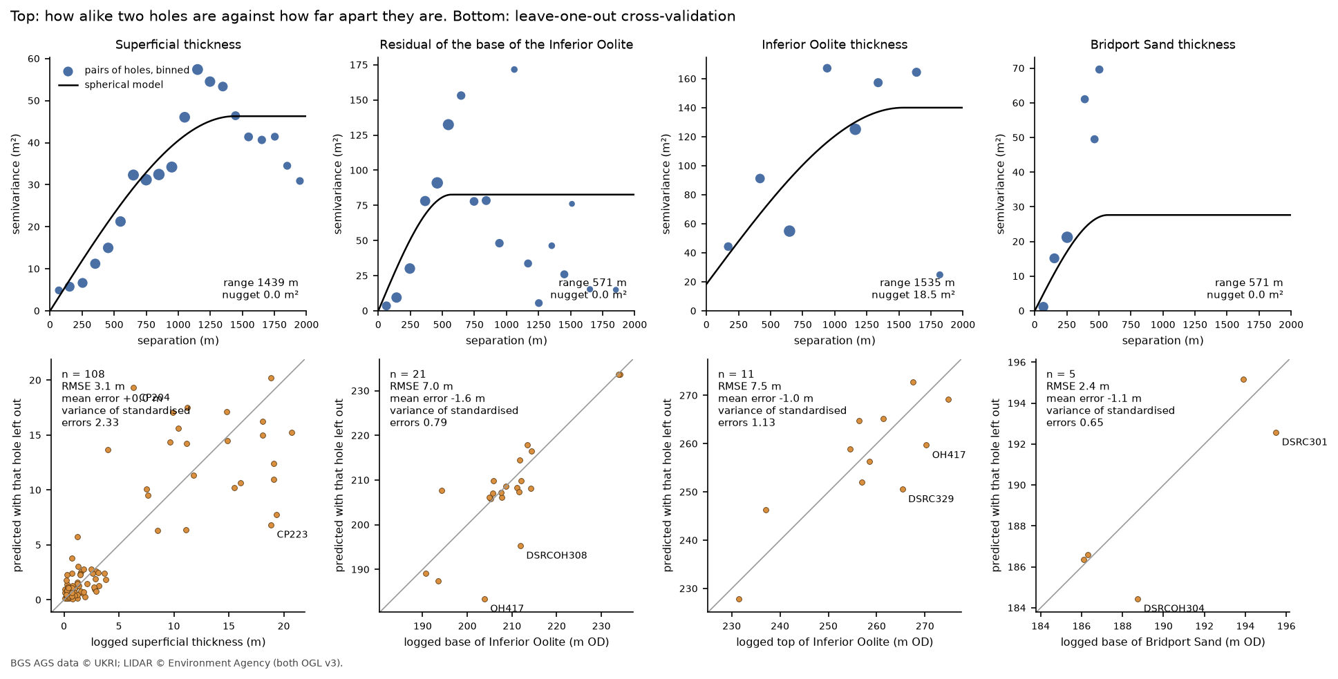
- Leave-one-out cross-validation gives each surface an honest error: 3.1 m for superficial thickness, 7.0 m for the base of the Inferior Oolite, 7.5 m for its top and 2.4 m for the base of the Bridport Sand.
- The three low holes Part 3 found at RC507 to RC509 are held out of the regional surface and modelled as their own small block. Kriging them in with everyone else makes the surface worse at the other 21 holes, from 7.01 m to 7.33 m.
Before you start
- Part 1 of this series, or at least its helper module a417_ags.py
- Python 3.10+ with python-ags4, PyKrige, SciPy, GeoPandas, rasterio, PyVista, requests and matplotlib
- Some familiarity with kriging helps: see Kriging spatial interpolation in Python
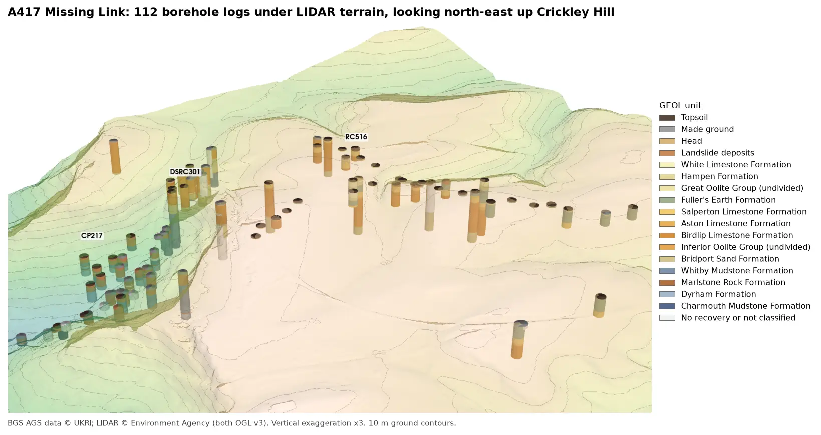
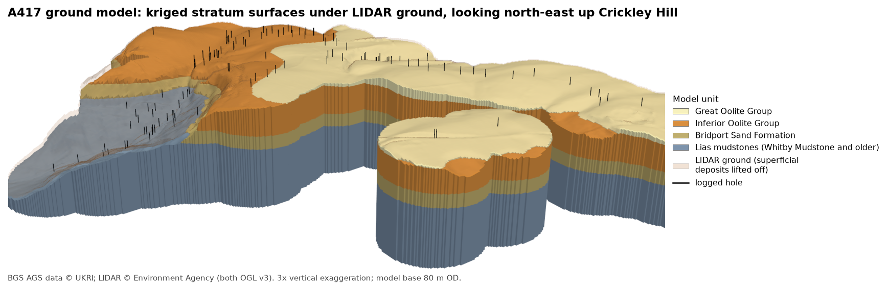
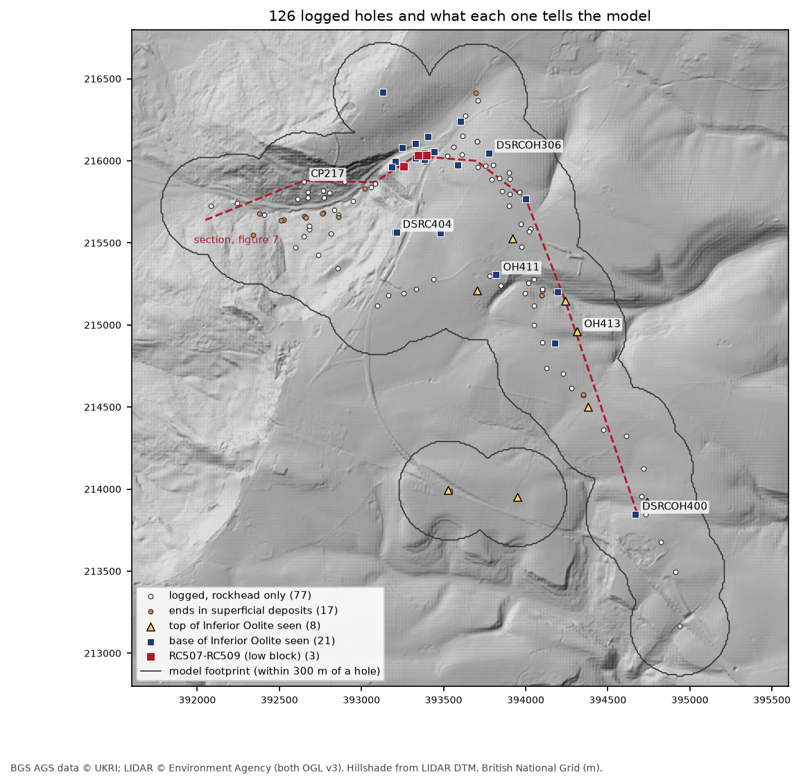
Boreholes tell you about the ground at a few points; a ground model fills in everything between them. In Part 3 we built every A417 log in 3D under the LIDAR terrain. Now we join them up: we pick four surfaces from the logs, krige each one onto a 10 m grid, and stack them under the LIDAR ground into a 3D model of the Cotswold escarpment at Crickley Hill.
An interpolated surface always looks convincing, which is exactly why it needs testing. So half of this part is evidence: how well each surface predicts holes it has not seen, where it is uncertain, whether it agrees with the holes that never reached it, and whether any surface crosses another. We also deal deliberately with the two places where Part 3 found the logs disagree with their neighbours, rather than letting the kriging smooth them away.
The steps are:
- collapse each log to five model units;
- pick the contacts, and turn holes that miss a surface into one-sided checks;
- fetch LIDAR ground and set up the model grid;
- krige rockhead;
- krige the base of the Inferior Oolite, with the low block at RC507 to RC509;
- hang the top of the Inferior Oolite and the base of the Bridport Sand from it;
- test the model;
- write the surfaces as GeoTIFFs;
- draw the figures and the 3D view.
The code is ground_model.py, which uses a417_ags.py from Part 1. It takes about four minutes, most of it cross-validation.
Step 1: collapse each log to five model units
Part 1 gave every GEOL interval a unit code, such as BLPL for the Birdlip Limestone or SLIP for landslide deposits. That is too fine for a ground model with 126 holes, so we group them into five units, youngest first:
GROUPS = {"SUP": ["TOPS", "MGR", "HEAD", "SLIP"], "GOG": ["WHL", "HMB", "GOG", "FE"], "IOG": ["SALS", "ASLS", "BLPL", "IOG"], "BDS": ["BDS"], "LIAS": ["WHM", "MRB", "DYS", "CHAM"]}The boundaries between them are the four surfaces we will model: rockhead (the base of the superficial deposits), the top of the Inferior Oolite, the base of the Inferior Oolite and the base of the Bridport Sand. Below that, the Lias mudstones run down to a flat base.
We use two BGS deposits this time. Item 173984 is the main ground investigation from Parts 1 to 3, and item 173975 adds 20 holes from a later phase on the crest of the escarpment, where the Inferior Oolite is thickest and least well known. Both go through Part 1’s download, merge and repair functions unchanged.
Part 3 found that CP217, in the landslide below the escarpment, logs Lias mudstone, then landslide debris, then Lias again: a slipped block of mudstone sitting on top of debris. Treated literally, that hole would put rockhead and the Lias at two levels. So, as Part 3 interpreted it, everything above 19.10 m in CP217 is counted with the landslide mass:
SLIPPED = {"CP217": 19.10} # Part 3: a slipped block repeats the Lias above this depthfor lid, depth in SLIPPED.items(): moved = (geol.LOCA_ID == lid) & (geol.GEOL_TOP < depth) & geol.group.notna() geol.loc[moved, "group"] = "SUP"Each log then collapses to a run of model units from top to bottom, and the script checks that no hole steps back to a younger unit further down:
=== Step 1: logs to model units ===CP217: 16 intervals above 19.1 m (a repeated Lias sequence) counted with the landslide mass132 holes from items 173984, 173975; 126 have at least one classified intervalholes whose model units step back to a younger unit: none“None” matters: it means that after the CP217 correction, every log is a simple sequence, and each surface can only be met once in each hole.
Step 2: pick the contacts, and what the other holes say
Where a hole passes from one unit to the next, the contact is at the midpoint of any unlogged gap between them. Most holes, though, never meet most surfaces. A shallow hole on the plateau that stops in Inferior Oolite says nothing about where the base is, except that it is below the bottom of the hole. A hole in the vale that starts in Lias mudstone tells us the Inferior Oolite has been eroded away there, so its base was above rockhead. These one-sided checks are free evidence, and we keep every one:
for s, (up, down) in BELOW.items(): a, b = r[r.group == up], r[r.group == down] if len(a) and len(b): # seen in the hole: the midpoint of any unlogged gap depth = (a.base.max() + b.top.min()) / 2 picks.append(dict(xy, surface=s, depth=depth, z=h.LOCA_GL - depth)) elif first_rock is not None and first_rock >= ORDER.index(down): # the hole starts in older rock, so this surface has been eroded and lay above rockhead bounds.append(dict(xy, surface=s, kind="above", z=h.LOCA_GL - rock.top.iloc[0])) elif len(rock) and ranks.max() <= ORDER.index(up): bounds.append(dict(xy, surface=s, kind="below", z=bottom)) # stops in older bedrock above itcontacts seen in the logs (holes): {'rockhead': 109, 'top_io': 11, 'base_io': 24, 'base_bds': 5}one-sided checks from holes that miss a surface:kind above below deeper thansurfacerockhead 0 0 17top_io 75 23 0base_io 24 61 0base_bds 24 80 0That is the shape of the problem in one table. Rockhead is seen in 109 holes, but the base of the Bridport Sand in only five, and the top of the Inferior Oolite in eleven. There are, though, 85 one-sided checks on the base of the Inferior Oolite and 104 on the base of the Bridport Sand, and we will use them all.
Step 3: LIDAR ground and the model grid
The top of the model is the Environment Agency’s LIDAR composite DTM, from the same Defra WCS as Parts 2 and 3. We fetch it at 5 m and average it to the 10 m model grid. The model only extends 300 m from a logged hole: further out, there is nothing to interpolate from.
=== Step 3: LIDAR ground and the model grid ===grid 400 x 400 cells of 10 m; 52,600 cells (5.26 km²) lie within 300 m of one of the 126 logged holeslogged ground level minus LIDAR at the holes: median -0.10 m, 90% within 0.75 mUsing LIDAR rather than each hole’s logged ground level keeps the top surface continuous between holes. The second line shows it is safe: the surveyed collar levels in LOCA agree with LIDAR to a median of 10 cm.
Step 4: rockhead
Rockhead follows the ground closely: its depth matters more than its elevation. So we krige the thickness of the superficial deposits and subtract it from the LIDAR ground. That way rockhead can never come out above the ground.
The variogram is fitted by hand rather than left to PyKrige. We bin every pair of holes by separation, weight each bin by its number of pairs, fit a spherical model with SciPy, and give the fitted parameters to OrdinaryKriging. This is the same approach as the kriging tutorial, with one difference: a fixed variogram lets us reuse it unchanged in cross-validation.
def fit_spherical(x, y, v, edges): """Fit a spherical variogram to the binned semivariances, weighting each bin by its number of pairs.""" lag, gam, n = experimental(x, y, v, edges) p, _ = curve_fit(spherical, lag, gam, p0=[gam.max(), edges[-1] / 3, 0], sigma=1 / np.sqrt(n), bounds=([0, edges[1], 0], [10 * gam.max(), edges[-1], gam.max()])) return dict(psill=p[0], range=p[1], nugget=p[2]), (lag, gam, n)Seventeen holes end in superficial deposits without reaching rock. Each one says the deposits are at least that thick. After the first kriging pass, honour() finds any such checks the surface breaks, adds those holes back as data at their limit, and kriges again until none are broken:
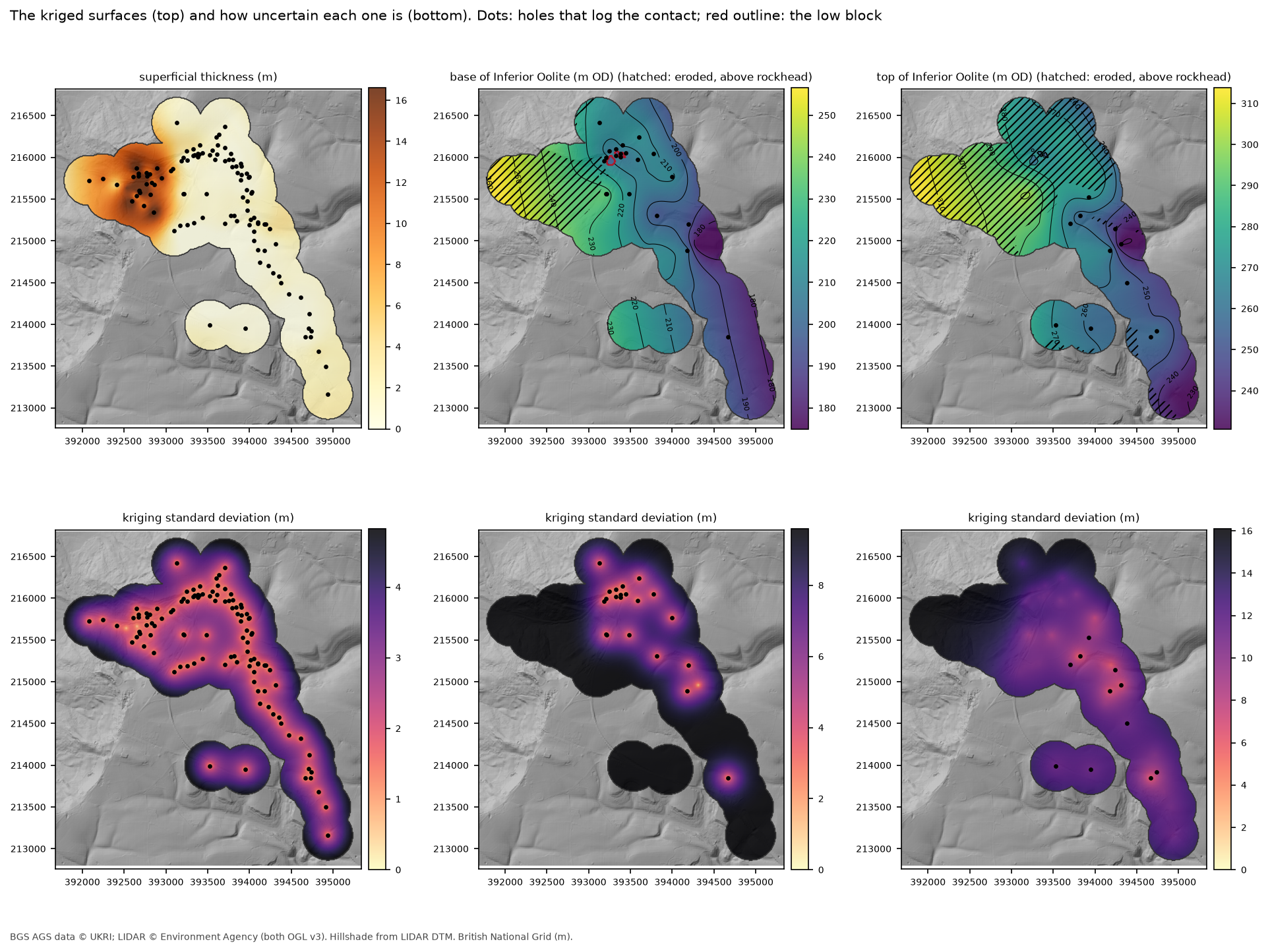
def honour(name, x, y, v, params, b, trend=False): """Krige, then turn every one-sided check the surface breaks into a data point at its limit, and repeat.""" added = np.zeros(len(b), bool) for _ in range(20): ex = b[added] f, coef = krige(np.r_[x, ex.x], np.r_[y, ex.y], np.r_[v, ex.limit], params, trend) m, _ = f(b.x.values, b.y.values) broken = np.where(b.kind == "above", m < b.limit - TOL, m > b.limit + TOL) & ~added if not broken.any(): break added |= broken=== Step 4: rockhead = LIDAR ground minus kriged superficial thickness === variogram: spherical, partial sill 46.3 m², range 1439 m, nugget 0.0 m² 108 thicknesses (after averaging repeat holes): median 1.00 m, max 20.70 m (CP208) one-sided checks: the first pass broke 3 of 17; 3 holes added at their limits; now broken: 0The median hole has a metre of topsoil and head over rock, but the landslide below the escarpment is up to 20.7 m thick, and the range of 1.4 km reflects that one large, deep area.
Step 5: the base of the Inferior Oolite, and the low block
The base of the Inferior Oolite is the backbone of the model. It is seen in 24 holes and has a clear regional dip, so we use regression kriging: fit a tilted plane, and krige only the residuals.
Part 3 found that three holes on top of the escarpment, RC507, RC508 and RC509, log this contact 11 to 15 m below their neighbours, with steep bedding and slickensides in the core: the signature of a cambered or foundered block, or possibly a small fault. If we krige them in with everyone else, the surface has to dive 15 m between holes 50 m apart, and the variogram has to treat that as noise. So they are held back from the regional surface:
CAMBER = ["RC507", "RC508", "RC509"] # Part 3: base of Inferior Oolite 11-15 m below neighboursbio = bio_all[~bio_all.LOCA_ID.isin(CAMBER)].reset_index(drop=True)res, coef = residuals(bio.x.values, bio.y.values, bio.z.values)=== Step 5: base of the Inferior Oolite: regional dip plus kriged residuals ===21 holes (RC507-RC509 held back). Fitted plane dips 1.33° (23.3 m per km) towards 76°; residuals -11.8 to +15.7 m variogram: spherical, partial sill 82.7 m², range 571 m, nugget 0.0 m² one-sided checks: the first pass broke 1 of 85; 1 holes added at their limits; now broken: 0 added: OH413A dip of just over 1° to the east is what the Cotswold dip slope should look like. The one hole added at its limit, OH413, is still in Inferior Oolite at 170.5 m OD: deeper than the first surface allowed, so the surface is pushed down to meet it.
Then we ask the regional surface where it expects the contact at the three low holes, and compare the evidence for keeping them out:
RC507-RC509 against the surface built from the other holes:LOCA_ID z regional sd offset RC507 197.90 210.34 3.97 -12.44 RC508 194.10 206.59 2.46 -12.49 RC509 190.15 205.07 2.20 -14.92kriging them in with the rest instead: LOOCV RMSE at the other 21 holes 7.33 m (without them 7.01 m); the variogram nugget rises from 0.0 to 13.9 m²low block: 114 cells (1.1 ha) lowered by 12.4 to 14.9 mEach offset is between three and seven of the surface’s own standard deviations, so the regional surface cannot explain them. Kriging them in makes the predictions at the other 21 holes worse, and adds a nugget of 13.9 m² to a variogram that otherwise has none. Both say the same thing: these holes are a separate piece of ground.
So we model them as one. Every cell that is nearer to one of the three than to any other hole on the contact, and within 60 m of it, is lowered by that hole’s offset:
d_good, _ = cKDTree(bio[["x", "y"]]).query(np.c_[gx.ravel(), gy.ravel()])d_cam, i_cam = cKDTree(cam[["x", "y"]]).query(np.c_[gx.ravel(), gy.ravel()])block = ((d_cam < d_good) & (d_cam <= 60)).reshape(ny, nx) & insidebase_io[block] += cam.offset.to_numpy()[i_cam.reshape(ny, nx)[block]]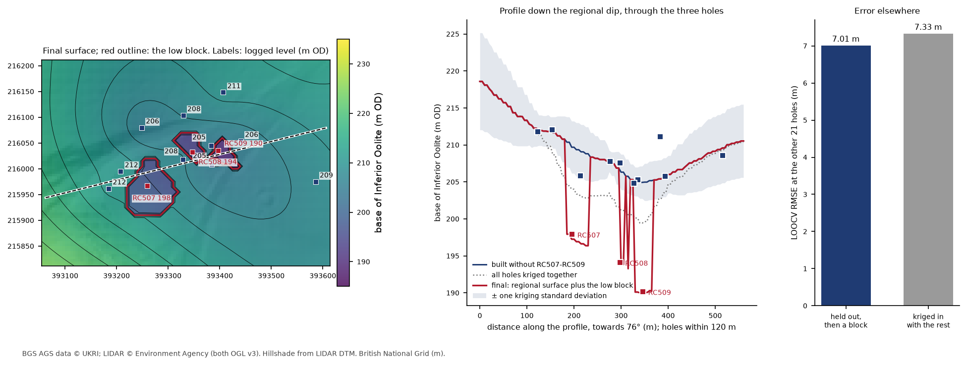
The block’s edges come from the nearest-hole rule. That is a modelling choice, not an observation: the logs show that the block exists, but not exactly where its edges are. Part 3’s alternative, a small fault, would give much the same surface at these holes.
Step 6: the top of the Inferior Oolite and the base of the Bridport Sand
Only 11 holes see the top of the Inferior Oolite and five the base of the Bridport Sand: far too few to krige either surface on its own. But both are much better known as thicknesses. The Inferior Oolite is 61 to 66 m thick in the four holes that go right through it, and the Bridport Sand is 16 to 28 m thick.
So we krige each thickness, an isochore, and hang it from the base of the Inferior Oolite. Where a hole sees the top but not the base, the thickness is measured from the modelled base:
tio["base_here"] = np.where(both, tio.LOCA_ID.map(bio_all.set_index("LOCA_ID").z), at(base_io, tio.E, tio.N))tio["thick"] = tio.z - tio.base_here...top_io = base_io + thick_iobase_bds = base_io - np.clip(thick_bds, 0, None) LOCA_ID z base_here thick through DSRC220 256.90 195.25 61.65 False DSRC329 265.35 188.04 77.31 False DSRC415 267.50 222.11 45.39 False DSRC420 256.35 210.33 46.02 FalseDSRCOH400 254.55 190.65 63.90 TrueDSRCOH412 237.10 187.87 49.23 False OH411 258.50 194.25 64.25 True OH413 231.45 170.49 60.96 False OH417 270.30 203.85 66.45 True RC516 274.75 201.98 72.77 False RC520 261.35 201.87 59.48 False variogram: spherical, partial sill 121.5 m², range 1535 m, nugget 18.5 m² one-sided checks: the first pass broke 15 of 98; 15 holes added at their limits; now broken: 0
Bridport Sand, 5 complete penetrations: DSRC109 18.2 m, DSRC301 16.3 m, DSRC319 24.8 m, DSRC408 28.1 m, DSRCOH304 17.0 m variogram: spherical, partial sill 27.6 m², range 571 m, nugget 0.0 m² one-sided checks: the first pass broke 5 of 104; 5 holes added at their limits; now broken: 0 added (holes that end in Bridport Sand below the first model): DSRC110, DSRC315, DSRC406, DSRC419, DSRCOH414modelled Bridport Sand thickness 16.4 to 37.1 mFive thicknesses cannot support a variogram of their own, so the Bridport Sand borrows the range of the base of the Inferior Oolite and takes their variance as its sill. The one-sided checks then do much of the work: five holes end in Bridport Sand below where the first model put its base, and pull it down. That is why the modelled thickness reaches 37 m, more than any hole proves.
The Inferior Oolite thickness checks matter just as much. The 75 holes that start in Great Oolite or Fuller’s Earth on the plateau each say the top of the Inferior Oolite is below them, and the first pass broke 15 of those. They are honoured in the final surface.
Step 7: does the model hold together?
Four tests, each answering a different question.
How well does each surface predict a hole it has not seen? Leave-one-out cross-validation takes each hole out, rebuilds the surface from the rest with the same variogram and one-sided checks, and predicts the missing hole:
def loocv(x, y, v, params, trend=False, extra=((), (), ())): """Leave each hole out in turn, rebuild from the rest (same variogram), and predict it.""" pred, sd = np.empty(len(v)), np.empty(len(v)) for i in range(len(v)): keep = np.arange(len(v)) != i f, _ = krige(np.r_[x[keep], extra[0]], np.r_[y[keep], extra[1]], np.r_[v[keep], extra[2]], params, trend) p, s = f(x[i:i + 1], y[i:i + 1]) pred[i], sd[i] = p[0], s[0] return pred, sd=== Step 7: does the model hold together? ===leave-one-out cross-validation (prediction minus log, m; standardised errors should average 0, variance 1): n RMSE mean_error MAE mean_SE var_SESuperficial thickness 108.0 3.09 -0.01 1.67 0.01 2.33Base of Inferior Oolite 21.0 7.01 -1.56 4.40 -0.21 0.79Top of Inferior Oolite 11.0 7.51 -0.96 6.60 -0.21 1.13Base of Bridport Sand 5.0 2.40 -1.08 1.81 -0.38 0.65The RMSE is the typical error in metres at an unseen hole. The standardised errors are each error divided by kriging’s own standard deviation at that hole. If the kriging uncertainties are honest, these average about 0 with a variance of about 1.
For the three bedrock surfaces they are close: the variances of 0.65 to 1.13 mean the standard deviation maps can be trusted. For superficial thickness the variance is 2.33, so the real errors are about one and a half times what kriging claims. That is the landslide: its thickness changes faster than one variogram for the whole site can describe. Read the superficial standard deviation map as a lower bound in the landslide area.
Do any surfaces cross? Building the top of the Inferior Oolite and the base of the Bridport Sand as thicknesses from its base should make that impossible, and the check confirms it in every one of the 52,600 cells:
no-crossing: top minus base of Inferior Oolite 44.3 to 70.7 m (0 cells cross); base of Inferior Oolite minus base of Bridport Sand 16.4 to 37.1 m; rockhead minus ground 0.0 m at mostDoes the model agree with the holes that never met a surface? Every one-sided check is tested against the final model, with half a metre of slack for the 10 m cells:
holes that miss a surface: does the model agree with them? holes agree worst_msurface kindrockhead deeper than 17 16 -0.9top_io above 75 71 -2.1 below 23 18 -4.2base_io above 24 24 26.6 below 61 61 -0.5base_bds above 24 23 -0.6 below 80 80 -0.1241 of 252 agree. The 11 that don’t miss by 4.2 m at most, and nine of them are on the top of the Inferior Oolite, the surface with the least data. honour() allows 1 m of slack when it adds holes, so these are holes it judged close enough at the time but that later steps moved slightly.
Is every unit where it should be? Finally, the surfaces are stacked from the top down with np.fmin. Where a younger surface is lower than an older one, the older unit has been eroded away there, and its surfaces take the younger level:
stack["top_io"] = np.fmin(top_io, stack["rockhead"])stack["base_io"] = np.fmin(base_io, stack["top_io"])stack["base_bds"] = np.fmin(base_bds, stack["base_io"])model base 80 m OD. Share of the model footprint where each unit is present: Superficial deposits 94%, Great Oolite Group 50%, Inferior Oolite Group 81%, Bridport Sand Formation 84%, Lias mudstones 100%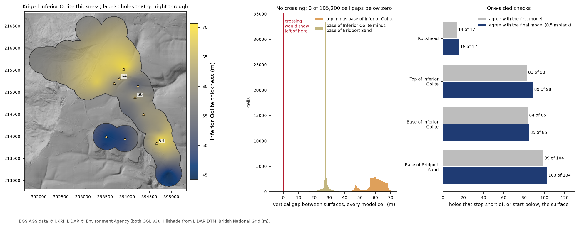
Step 8: write the surfaces
Each surface, and each standard deviation, goes to a GeoTIFF in British National Grid, along with a small model.json that records the units, their colours and which surface is the top and base of each. That is all Part 7 needs to turn the model into a print, and the GeoTIFFs open directly in QGIS.
=== Step 8: write the surfaces ===wrote base_bridport_sand_mOD.tif, base_inferior_oolite_mOD.tif, ground_mOD.tif, low_block.tif, model.json, rockhead_mOD.tif, sd_base_bridport_sand_mOD.tif, sd_base_inferior_oolite_mOD.tif, sd_rockhead_mOD.tif, sd_top_inferior_oolite_mOD.tif, top_inferior_oolite_mOD.tif and loocv.csvloocv.csv holds every cross-validated prediction, so you can map the errors yourself.
Step 9: the section and the 3D view
A section along the route corridor is the best single test of a ground model, because it puts the surfaces and the logs side by side:
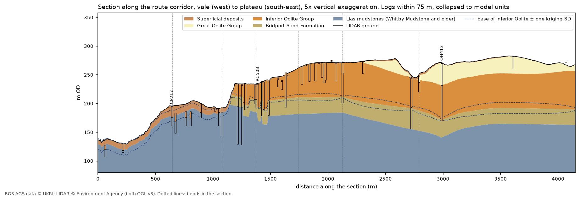
The low block shows as a narrow notch in the base of the Inferior Oolite at RC508. Further east, the Inferior Oolite dips to its lowest point at OH413, where the hole is still in limestone at 170 m OD; we come back to that below.
The 3D view at the top of the page is built in PyVista. Each unit is a solid between its top and base surfaces, made by stacking two StructuredGrids and extracting the outer surface, and the logged holes are drawn as lines. The superficial deposits are drawn as a thin, faint skin on top, so that the bedrock geology, which is what the model is mostly about, shows through.
Frequently asked questions
How do I build a geological model from borehole data in Python?
Pick each contact from the logs, krige the best-sampled surface first, and build the others from it as kriged thicknesses, so they cannot cross. Stack them under a ground surface such as LIDAR, using np.fmin so eroded units take the level of the surface above them. PyKrige does the kriging; NumPy and rasterio handle the grids.
Why krige thickness rather than elevation?
Thickness usually varies more gently than elevation, and adding a kriged thickness to a surface guarantees the two never cross. It also lets holes that only see one contact still contribute, by measuring their thickness from the modelled surface below.
What do I do with boreholes that don’t reach a surface?
Use them as one-sided checks: a hole that stops above a surface says the surface is below it. Krige without them, find any the surface breaks, add those as data at their limit, and krige again. Here, 252 such checks shaped the model, and the final surfaces agree with all but 11 of them.
How accurate is a kriged ground model?
Leave-one-out cross-validation gives the honest answer for your site. Here the typical error at an unseen hole is 3 m for superficial thickness and 7 to 7.5 m for the Inferior Oolite surfaces, which is large compared with the 2 to 3 m kriging standard deviation near the holes, and small compared with a 60 m thick formation.
What should I do when one borehole disagrees with its neighbours?
First check the log, as Part 3 did. If the disagreement is real geology, such as a slipped or let-down block, take the hole out of the regional surface and model the block on its own. Cross-validation tells you whether that is the right call: here it improved the predictions everywhere else.
Next steps
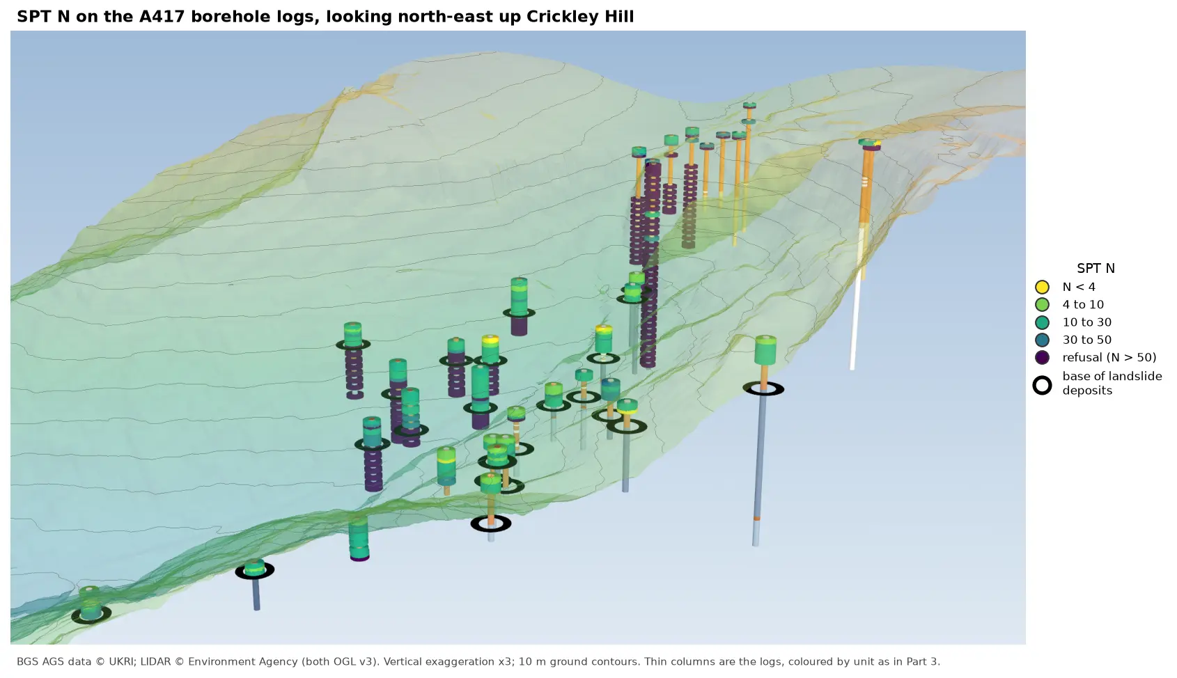
- Part 6: SPT N-values shows how hard each unit is, and how sharply the ground stiffens at the base of the landslide deposits.
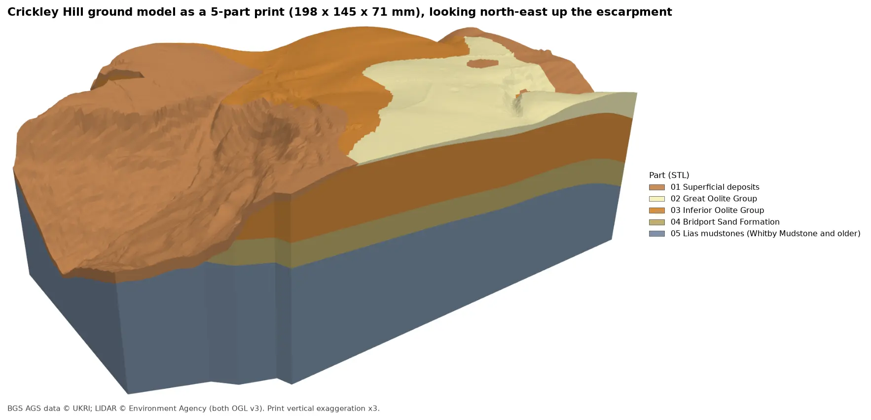
- Part 7: 3D-print the ground model turns these surfaces into one watertight STL per unit for a multi-material printer.
- Kriging spatial interpolation in Python explains variograms and kriging from the start, and compares kriging with simpler interpolators.
- 3D terrain visualisation with PyVista covers PyVista lighting and cameras in more depth.
- Back to Part 3: 3D borehole logs, where the low block at RC507 to RC509 was first found.
Data and licences
- A417 Missing Link ground investigation (BGS deposited data items 173984 and 173975; client Highways England, now National Highways), downloaded through the BGS AGS borehole index and export APIs. Contains British Geological Survey materials © UKRI 2026, licensed under the Open Government Licence v3.0.
- Environment Agency LIDAR Composite DTM 1 m, requested at 5 m from the Defra Data Services Platform WCS. © Environment Agency copyright and/or database right, licensed under the Open Government Licence v3.0. It is the ground surface of the model and the hillshade in every map, and each figure carries the credit. No third-party web map tiles are used.
- Code:
ground_model.pyanda417_ags.py, tested with Python 3.12.0, python-ags4 1.2.0, PyKrige 1.7.3, SciPy 1.18.1, NumPy 2.5.4, rasterio 1.5.2, PyVista 0.49.2 and VTK 9.7.2.
Key terms
- Ground model
- A 3D description of the layers beneath a site, built here as a stack of surfaces, each the base of one unit and the top of the next.
- Rockhead
- The top of bedrock: the base of the superficial deposits such as topsoil, made ground, head and landslide debris.
- Isochore
- A map of the vertical thickness of a unit. Kriging a thickness and adding it to a surface below guarantees the two surfaces never cross.
- Regression kriging
- Fitting a trend, here a tilted plane for the regional dip, and kriging only what is left over. The final surface is the plane plus the kriged residuals.
- Leave-one-out cross-validation
- Taking each borehole out in turn, rebuilding the surface from the rest and predicting it. The differences show how well the model predicts ground it has not seen.
- Kriging standard deviation
- Kriging's own estimate of its uncertainty at every cell. It grows with distance from the holes and depends on the variogram, not on the values themselves.
Data for this tutorial
- BGS AGS borehole data · Donated AGS ground investigation data, Open Government Licence
Licences and formats for each source are listed in the GIS data sources catalogue.