Visualising SPT N-values from AGS4 data in Python
Read the Standard Penetration Tests (ISPT) from a real AGS4 file, separate full tests from refusals, find the stratum each test was made in, and show the N-values four ways: by unit against elevation, across the base of a landslide, as coloured discs on 3D borehole logs over LIDAR terrain, and as a map of the depth to the first refusal.
- Level
- Intermediate
- Tested with
- Python 3.12
- Source code
- Download scripts
Key takeaways
- The AGS4 ISPT group gives each test's depth and reported N. Tests that hit 50 blows before the full 300 mm are refusals, and this file reports them as N scaled up to 300 mm, so values run to 1,200. Treat anything above 50 as a refusal, not as a measurement.
- Joining each test to the GEOL interval that contains it turns a list of blow counts into evidence about the ground. On the A417, median N rises from 19 in the landslide deposits to over 100 in every bedrock unit below them.
- Plotting N against height above or below the logged base of the landslide deposits shows how sharp that contact is: 5% of tests refuse above it and 84% below it.
- The depth to the first refusal maps the thickness of soft ground. It is 2.2 m (median) on the limestone plateau and 13.0 m on the escarpment, where the landslide deposits are thickest.
Before you start
- Part 1 of this series, or at least its helper module a417_ags.py
- Python 3.10+ with python-ags4, pandas, GeoPandas, rasterio, PyVista, requests and matplotlib
- Part 3 is useful background for the 3D view
A borehole log tells you what the ground is; the SPTs tell you how hard it is. In Part 3 we built the A417 Missing Link logs in 3D, and in Part 5 we interpolated them into a ground model. This part adds the 415 Standard Penetration Tests in the same file and asks a simple question of them: where does the soft ground stop?
On Crickley Hill the answer is mostly at the base of the landslide deposits that cover the escarpment. The figures below show that from four directions, and every number in them comes straight from the AGS file.
The steps are:
- read the SPTs and pick out the refusals;
- find the GEOL unit each test was made in;
- plot N against elevation for each unit;
- plot N across the base of the landslide deposits;
- put the N-values on the 3D logs over LIDAR terrain;
- map the depth to the first refusal;
- write the tests to a GeoPackage for QGIS.
The code is spt_n_values.py. It uses a417_ags.py from Part 1, which downloads and repairs the AGS file the first time it runs.
Step 1: read the SPTs and pick out the refusals
AGS4 keeps SPT results in the ISPT group. In this file it has four columns: LOCA_ID, the depth to the top of the test (ISPT_TOP), the reported N (ISPT_REP) and an empty hammer reference (ISPT_HAM). There is no record of the seating drive, the blows for each 75 mm, or the hammer’s energy ratio, so we work with N as reported.
spt = ags["ISPT"][["LOCA_ID", "ISPT_TOP", "ISPT_REP"]].copy()spt["ISPT_TOP"] = pd.to_numeric(spt.ISPT_TOP)spt["N"] = pd.to_numeric(spt.ISPT_REP)spt["refusal"] = spt.N > 50spt["pen_mm"] = np.where(spt.refusal, 50 * 300 / spt.N, 300.0) # penetration implied by 50 blowsspt = spt.join(loca[["LOCA_NATE", "LOCA_NATN", "LOCA_GL"]], on="LOCA_ID")spt["mOD"] = spt.LOCA_GL - spt.ISPT_TOP=== Step 1: SPT N-values and refusals ===415 tests in 52 holes, 0.6 to 105.0 m deepN from 2 to 1200; 183 tests (44%) above 50penetration implied by those values for 50 blows: 12.5 to 294.1 mm, e.g. 12, 47, 80, 123, 200, 294N runs to 1,200, which no test can actually reach. A test stops after 50 blows in the main drive, so any N above 50 is a refusal that the contractor has scaled up to 300 mm. Turning it back into the penetration it implies, 50 × 300 / N, gives 12.5 to 294 mm: an N of 1,200 means the sampler moved 12.5 mm in 50 blows. That is useful as a ranking of how hard the ground was, but not as a measurement, so every chart below shades N above 50 grey and draws refusals as triangles.
Step 2: find the GEOL unit each test was made in
An N-value means little without the ground it was measured in. Join each test to its hole’s GEOL intervals and keep the interval whose top and base bracket the test depth:
g = geol[["LOCA_ID", "GEOL_TOP", "GEOL_BASE", "UNIT"]]m = spt.reset_index().merge(g, on="LOCA_ID", how="left")m = m[(m.GEOL_TOP <= m.ISPT_TOP) & (m.ISPT_TOP < m.GEOL_BASE)].drop_duplicates("index").set_index("index")spt["UNIT"] = m.UNIT.reindex(spt.index).fillna("NR")=== Step 2: the GEOL unit at each test === tests holes median_N refusalsUNITMGR 7 3 5.0 0%HEAD 13 9 18.0 8%SLIP 189 31 19.0 5%WHL 3 2 150.0 100%HMB 1 1 171.0 100%FE 18 6 23.0 28%ASLS 1 1 600.0 100%BLPL 38 11 106.0 68%BDS 31 6 231.0 94%WHM 73 10 316.0 97%MRB 1 1 316.0 100%DYS 26 7 131.5 96%CHAM 2 1 24.0 0%NR 12 11 218.0 92%The UNIT codes are the ones a417_ags.py gives each GEOL description in Part 1. Nearly half of all the tests, 189, were made in the landslide deposits (SLIP). Their median N of 19 is close to that of the made ground, head and Fuller’s Earth clay. Every bedrock unit below them has a median above 100, and most of their tests refused. NR is where the log records no recovery, typically because the ground was too hard to sample, and 92% of those tests refused too.
Step 3: N against elevation, by unit
A chart for each unit, with elevation on the vertical axis and N on a log scale, shows both how hard each unit is and where it sits in the hill:
for ax, u in zip(axes, facets + ["other"]): d = spt[spt.UNIT == u] if u != "other" else spt[~spt.UNIT.isin(facets)] ax.axvspan(50, 2000, color="#eeeeee", zorder=0) for refused, marker in [(False, "o"), (True, ">")]: e = d[d.refusal == refused] ax.scatter(e.N, e.mOD, c=[A.UNITS.colour[x] for x in e.UNIT], marker=marker, s=22 if refused else 16, edgecolor="#333333", lw=0.4, zorder=3) ax.set_xscale("log")=== Step 3: N against elevation, by unit ===Made ground 7 tests median N 5 168 to 192 m ODHead 13 tests median N 18 229 to 278 m ODLandslide deposits 189 tests median N 19 120 to 254 m ODFuller's Earth 18 tests median N 23 243 to 285 m ODBirdlip Limestone 38 tests median N 106 212 to 267 m ODBridport Sand 31 tests median N 231 189 to 212 m ODWhitby Mudstone 73 tests median N 316 129 to 194 m ODDyrham 26 tests median N 132 139 to 179 m ODOther units 20 tests median N 214 128 to 281 m OD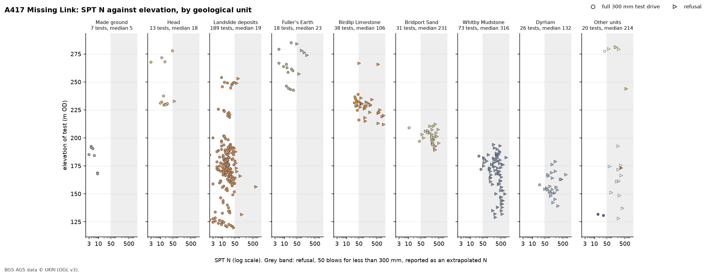
Two things stand out. The first is the split between the soft units on the left and the bedrock units on the right. The second is the landslide deposits’ spread of elevation. Every other unit sits in a narrow band of height, as layers in a hill should, but the landslide deposits are found over 134 m of it, because they lie on the slope rather than in the sequence.
What the N-values mean depends on the ground. BS EN ISO 14688-2 and BS 5930 use N to describe the density of sands and gravels: under 4 is very loose, 4 to 10 loose, 10 to 30 medium dense, 30 to 50 dense and over 50 very dense. The bands in the 3D view and the map follow those limits. Here they apply strictly only to the Bridport Sand, which is very dense. The clays and weak rocks are described by strength instead, and N is one guide to that among others, so treat the bands there as a scale of hardness.
Step 4: N across the base of the landslide deposits
If the landslide deposits are soft and the bedrock is hard, the change should happen at the contact between them. To test that, take every hole that logs landslide deposits directly on bedrock and measure each test’s height above or below that hole’s contact:
rows = []for lid, h in geol.groupby("LOCA_ID"): s = h[h.UNIT == "SLIP"] if s.empty: continue under = h[(h.GEOL_TOP >= s.GEOL_BASE.max() - 0.01) & h.UNIT.isin(bedrock)] if len(under): rows.append((lid, s.GEOL_BASE.max(), under.UNIT.iloc[0]))base = pd.DataFrame(rows, columns=["LOCA_ID", "slip_base", "below"]).set_index("LOCA_ID")b = spt.join(base, on="LOCA_ID", how="inner")b["rel"] = b.slip_base - b.ISPT_TOP # metres above (+) or below (-) the logged base=== Step 4: across the base of the landslide deposits ===31 holes log landslide deposits directly on bedrock; 28 of them have SPTs (235 tests)base of the deposits: 1.3 to 20.7 m deep, median 10.4 mabove the base: 178 tests, median N 19, refusals 5%below the base: 57 tests, median N 128, refusals 84%first test below the base refused in 7 of 12 holes; bedrock beneath: Whitby Mudstone Formation 15, Dyrham Formation 5, Charmouth Mudstone Formation 3, Salperton Limestone Formation 3, Fuller's Earth Formation 3, Marlstone Rock Formation 1, Aston Limestone Formation 1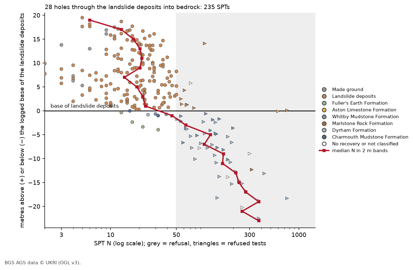
The base of the landslide deposits is where the ground gets hard. Above it, the median N is between 13 and 24 in every 2 m band up to 18 m above the contact. Only 9 of the 178 tests refuse, and 5 of those are within 1.5 m of the base. Below it, the median jumps to 128 and 84% refuse. The first test below the contact refused in 7 of the 12 holes that have one.
That is good evidence that the loggers placed the contact well. It also shows that the landslide deposits are soft right down to their base, rather than stiffening gradually with depth. Most of them, 15 of 31 holes, rest on Whitby Mudstone.
Step 5: N on the 3D logs over LIDAR
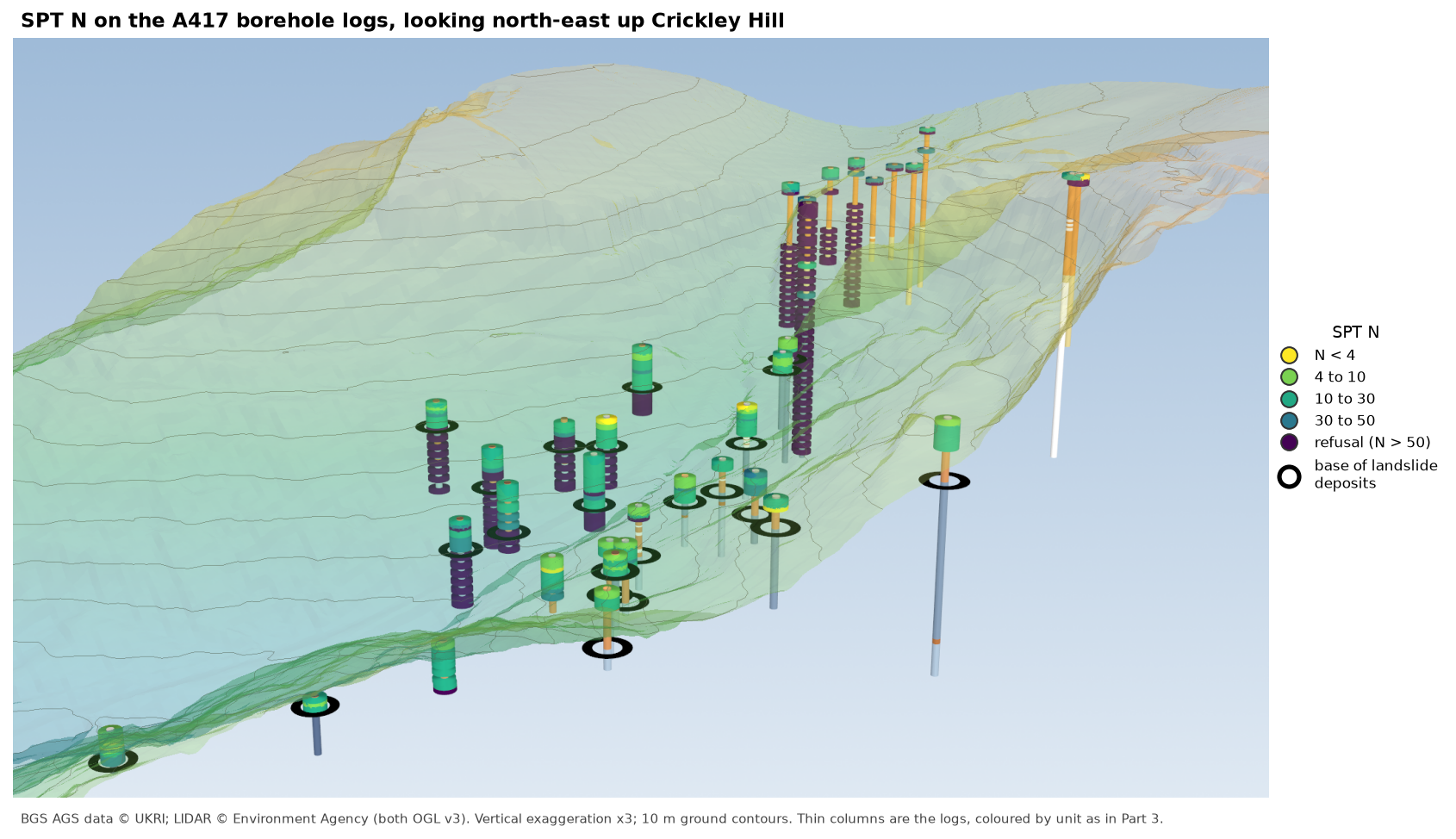
The lead figure puts the same tests where they were made. It reuses Part 3’s approach: thin cylinders for the GEOL intervals, coloured by unit, under semi-transparent LIDAR terrain at three times vertical exaggeration. Each SPT becomes a wider, flat disc at its elevation, coloured by its N band, and each hole from Step 4 gets a black ring at the base of its landslide deposits:
discs = [coloured(pv.Cylinder(center=(r.LOCA_NATE - X0, r.LOCA_NATN - Y0, r.mOD * VE), direction=(0, 0, 1), radius=11, height=1.4 * VE, resolution=32), BAND_COLOURS[int(r.band)]) for r in spt[spt.LOCA_ID.isin(holes.index)].itertuples()]rings = [pv.Disc(center=(loca.at[lid, "LOCA_NATE"] - X0, loca.at[lid, "LOCA_NATN"] - Y0, (loca.at[lid, "LOCA_GL"] - d) * VE + 0.5), inner=13, outer=22, normal=(0, 0, 1), c_res=48) for lid, d in base.slip_base.items() if lid in holes.index]=== Step 5: N on the 3D logs ===39 holes with SPTs on Crickley Hill: 880 log intervals, 378 SPT discs, 24 rings at the base of the landslide depositsThe colours come from viridis, from yellow for very low N to dark purple for refusals, so the change from soft to hard reads as a change from light to dark even in greyscale. In the view at the top of the page, the holes on the escarpment are green above their black rings and purple below them, and the holes on the plateau at the top right turn purple almost at the surface.
Step 6: map the depth to the first refusal
The 3D view shows a pattern; a map measures it. For each hole, find the shallowest test that refused. Holes that never refused are shown as white circles labelled with the depth of their deepest test, because that is as far as we know the ground stayed soft:
first = spt[spt.refusal].groupby("LOCA_ID").ISPT_TOP.min()none = spt.groupby("LOCA_ID").ISPT_TOP.max()[~spt.groupby("LOCA_ID").refusal.any()]=== Step 6: depth to the first refusal ===32 holes reached refusal, at 0.6 to 60.0 m (median 4.1 m); 20 holes never did (deepest test 1.0 to 13.7 m) plateau, east of 393,100 E: 9 holes, median depth to refusal 2.2 m escarpment, west of 393,100 E: 11 holes, median depth to refusal 13.0 m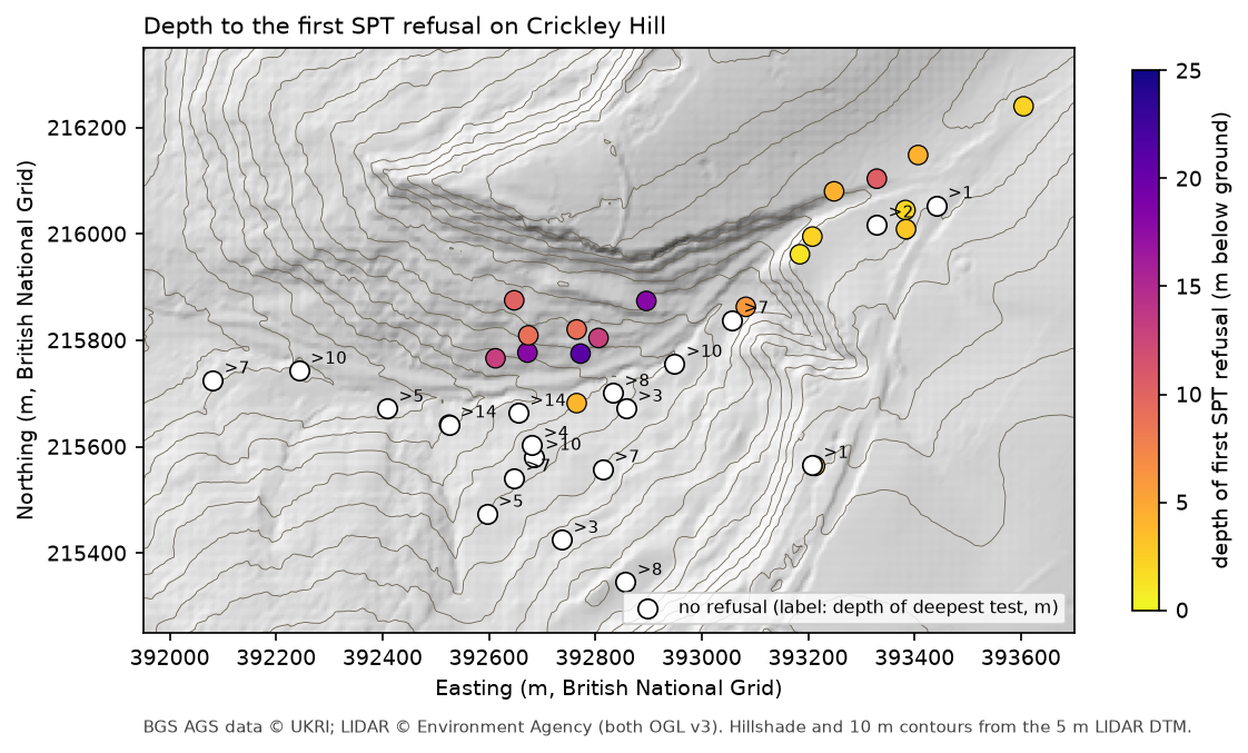
The map divides the hill into three. On the plateau, the Birdlip Limestone is within a few metres of the surface under a metre or two of head or made ground, and 8 of the 9 plateau holes first refused in it, at a median depth of 2.2 m. On the escarpment face the median is 13.0 m: 5 of those 11 holes first refused in the landslide deposits and 6 in the Lias mudstones beneath them. Most of the holes that never refused, 14 of 20, are on the lower slopes and in the vale to the south-west, and their deepest test was still in the landslide deposits.
Step 7: write the tests to a GeoPackage for QGIS
The same table, with a PointZ geometry at each test’s position and elevation, goes into a GeoPackage. You can add it to the QGIS project from Part 2, style it by band, or show it in the 3D map view from Part 3:
pts = gpd.GeoDataFrame( spt[["LOCA_ID", "ISPT_TOP", "mOD", "N", "refusal", "pen_mm", "UNIT"]] .assign(unit_name=spt.UNIT.map(A.UNITS.name), band=[BAND_LABELS[int(i)] for i in spt.band]), geometry=gpd.points_from_xy(spt.LOCA_NATE, spt.LOCA_NATN, spt.mOD), crs="EPSG:27700")pts.to_file(OUT / "a417_spt.gpkg", layer="spt", driver="GPKG")=== Step 7: write the tests to a GeoPackage ===a417_spt.gpkg: 415 PointZ features in EPSG:27700, fields LOCA_ID, ISPT_TOP, mOD, N, refusal, pen_mm, UNIT, unit_name, bandfigures: 01-spt-n-3d.png, 02-n-vs-elevation-by-unit.png, 03-n-across-slip-base.png, 04-depth-to-refusal-map.pngFrequently asked questions
Where are SPT results in an AGS4 file?
In the ISPT group, one row for each test, keyed by LOCA_ID and the depth to the top of the test, ISPT_TOP. The N-value is in ISPT_NVAL, and ISPT_REP holds the result as the contractor reported it, which may be text such as “50/75” or, as here, an extrapolated N. Penetration (ISPT_NPEN), seating and main-drive blows, the 75 mm increments and the hammer energy ratio have their own headings if the contractor supplied them.
How should I plot SPT refusals?
Keep them, but mark them differently. Refusals are often the most informative tests because they show where hard ground starts. Plot them with their own symbol and shade the region above N = 50, rather than mixing extrapolated values with measured ones or dropping them.
Is this N60?
No. N60 needs the energy ratio of the hammer used, and this file has neither ISPT_ERAT nor ISPT_N60, and an empty hammer reference. The values here are N as reported. For design you would correct for hammer energy, and for overburden pressure in sands, using the contractor’s hammer calibration records.
Why use a log scale for N?
Measured N on this site runs from 2 to 50, and extrapolated refusals go to 1,200. On a linear scale everything below 50 is squeezed against the axis. A log scale gives the soft ground room and still shows the refusals.
Can I do this with any AGS file?
Yes. Steps 1, 2, 3, 6 and 7 need only LOCA, GEOL and ISPT. Step 4 needs a contact that many holes pass through, so swap SLIP for the base of made ground, alluvium or glacial till on your site.
Next steps
- Part 7: 3D-print the ground model turns the kriged surfaces from Part 5 into a multi-material print of Crickley Hill.
- Part 4: a geological cross-section is a good place to add the N-values from Step 7 along the section line.
- Kriging spatial interpolation in Python shows how you could turn the depth to first refusal into a continuous surface.
- Back to Part 1: Reading and validating AGS4 files, Part 2: Boreholes on a map, Part 3: 3D borehole logs or Part 5: the ground model.
Data and licences
- A417 Missing Link ground investigation (BGS deposited data item 173984; client Highways England, now National Highways; contractor Geotechnical Engineering Ltd), downloaded through the BGS AGS borehole index and export APIs. Contains British Geological Survey materials © UKRI 2026, licensed under the Open Government Licence v3.0. Every figure carries the credit.
- Environment Agency LIDAR Composite DTM 1 m, requested at 5 m from the Defra Data Services Platform WCS. © Environment Agency copyright and/or database right, licensed under the Open Government Licence v3.0. It is the terrain in the 3D view and the hillshade and contours in the map, and both figures carry the credit. No other basemap is used.
- Code:
spt_n_values.pyanda417_ags.py, tested with Python 3.12.0, python-ags4 1.2.0, pandas 2.3.3, GeoPandas 1.2.0, rasterio 1.5.2, PyVista 0.49.2, VTK 9.7.2 and matplotlib 3.11.2.
Key terms
- Standard Penetration Test (SPT)
- An in-situ test in which a 63.5 kg hammer falling 760 mm drives a split-spoon sampler or solid cone into the bottom of a borehole. After a 150 mm seating drive, the blows for the next 300 mm are the N-value.
- N-value
- The number of blows to drive the sampler 300 mm after the seating drive. Low N means loose or soft ground and high N means dense or hard ground.
- Refusal
- A test stopped after 50 blows in the main drive before the sampler has gone the full 300 mm. The penetration reached is recorded, and some contractors report an N extrapolated to 300 mm.
- N60
- N corrected to 60% of the hammer's theoretical energy, so tests with different hammers can be compared. It needs the hammer's measured energy ratio, which this file does not hold.
- Landslide deposits
- Ground that has slid down a slope, here mainly Lias clay and broken limestone that has moved off the Cotswold escarpment. Its base is often a polished slip surface on undisturbed bedrock.
Data for this tutorial
- BGS AGS borehole data · Donated AGS ground investigation data, Open Government Licence
Licences and formats for each source are listed in the GIS data sources catalogue.