3D borehole logs from AGS4 data in PyVista and QGIS
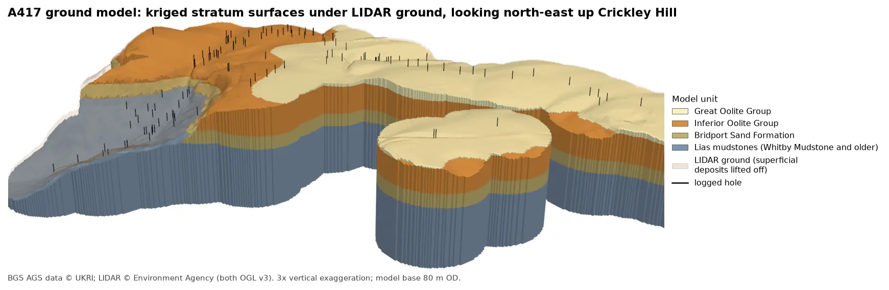
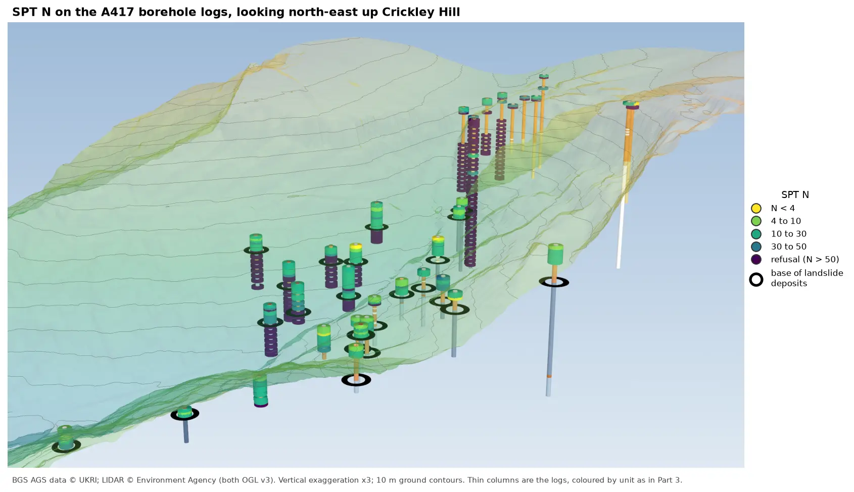
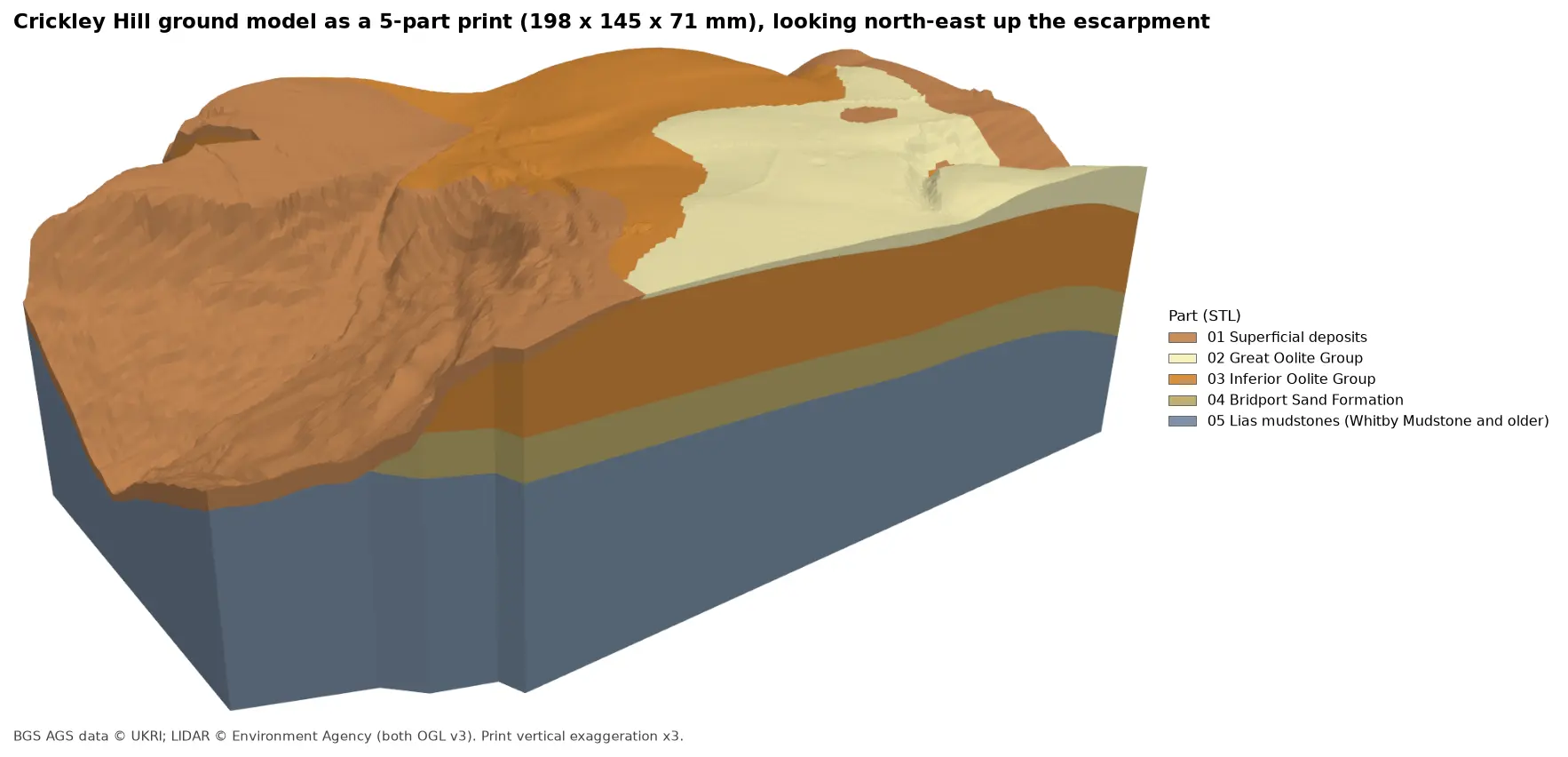
Build every borehole log in a real AGS4 file as coloured 3D cylinders at their true elevation under Environment Agency LIDAR terrain with PyVista, then style the same intervals in the QGIS 3D map view. Along the way, test whether neighbouring logs agree, and find a block of ground at the top of Crickley Hill where they don't.
- Level
- Intermediate
- Tested with
- Python 3.12
- Source code
- Download scripts
Key takeaways
- Each GEOL interval becomes a cylinder from ground level minus its top depth to ground level minus its base depth. Merging all 1,564 into one mesh keeps PyVista fast.
- Giving every face an RGB colour from a single unit table keeps the PyVista view, the strip logs and the QGIS style consistent.
- Neighbouring logs are evidence for each other. Close pairs of holes agree on the base of the Inferior Oolite to a median of 1.1 m, except three holes on top of Crickley Hill that record it 11 to 15 m lower, alongside steep bedding and slickensides.
- QGIS can show the same logs in its 3D map view as extruded prisms styled with one rule per unit, against LIDAR terrain cut away in front of them.
Before you start
- Part 1 of this series, or at least its helper module a417_ags.py
- Python 3.10+ with python-ags4, PyVista, GeoPandas, rasterio, shapely, requests and matplotlib
- QGIS 3.34 or later for the 3D map view (tested with 3.40 LTR)
A map shows where the boreholes are; a 3D view shows what they found. In Part 1 we read and repaired the A417 Missing Link ground investigation, and in Part 2 we put its 112 holes on a map. Now we build every log in 3D, at its true elevation under the LIDAR terrain, so you can see the Jurassic layers of the Cotswold escarpment the way the drillers met them.
A 3D view is also a good way to check the data. If neighbouring logs disagree, it shows straight away, and the second half of this part follows up one place where they do.
The steps are:
- give every GEOL interval an elevation;
- fetch the LIDAR terrain;
- build the strata cylinders;
- render the overview in PyVista;
- check whether neighbouring logs agree;
- write 3D lines for QGIS and style them in its 3D map view.
The code is borehole_logs_3d.py for Steps 1 to 6 and qgis_3d_logs.py for the QGIS project. Both use a417_ags.py from Part 1.
Step 1: give every GEOL interval an elevation
GEOL records depths below ground. LOCA records the ground level and position of each hole. Join the two on LOCA_ID, subtract, and every interval has a top and base in metres above Ordnance Datum:
ags = A.load_clean(DATA)loca = ags["LOCA"].set_index("LOCA_ID")geol = ags["GEOL"].copy()geol["UNIT"] = geol.UNIT.fillna("NR")geol = geol.join(loca[["LOCA_NATE", "LOCA_NATN", "LOCA_GL"]], on="LOCA_ID")geol["top_mOD"] = geol.LOCA_GL - geol.GEOL_TOPgeol["base_mOD"] = geol.LOCA_GL - geol.GEOL_BASEgeol["thick"] = geol.GEOL_BASE - geol.GEOL_TOPgeol = geol[geol.thick > 0].reset_index(drop=True)=== Step 1: GEOL intervals with elevations ===1564 intervals in 112 holes | 3,299 m of logged ground | elevations 107.5 to 294.1 m OD intervals holes metresUNITTOPS 66 66 17.0MGR 85 36 33.6HEAD 54 34 33.8SLIP 320 41 375.9WHL 11 4 23.8HMB 21 9 36.6GOG 7 5 3.1FE 156 28 302.1SALS 63 21 145.5ASLS 25 20 35.0BLPL 322 34 1026.0IOG 1 1 2.0BDS 101 22 354.5WHM 125 20 418.0MRB 12 10 11.0DYS 109 16 164.7CHAM 20 3 31.4NR 66 24 285.7The Birdlip Limestone dominates, with over a kilometre of core in 34 holes. That is the thick limestone the new road cuts through on the climb up the escarpment. The 376 m of landslide deposits in 41 holes is a reminder of how much of the slope below it has moved.
Step 2: fetch the LIDAR terrain
As in Part 2, the terrain comes from the Environment Agency’s LIDAR composite DTM through the Defra WCS, this time as one request at 5 m resolution, which is plenty under 112 holes. PyVista draws it as a StructuredGrid. Coordinates are measured from the corner of the area, so the numbers stay small for the graphics card, and heights are multiplied by the vertical exaggeration VE:
xs = left - X0 + RES / 2 + np.arange(dtm.shape[1]) * RESys = top - Y0 - RES / 2 - np.arange(dtm.shape[0]) * RESgx, gy = np.meshgrid(xs, ys)z = np.nan_to_num(dtm, nan=np.nanmin(dtm))terrain = pv.StructuredGrid(gx, gy, z * VE)terrain["elevation"] = z.ravel(order="F")=== Step 2: LIDAR terrain ===DTM 800 x 800 cells of 5 m, 81.8 to 302.9 m ODIf you have not used PyVista with terrain before, 3D terrain visualisation with PyVista covers the basics.
Step 3: build the strata cylinders
Each interval becomes a short cylinder, centred halfway between its top and base and as tall as it is thick. Rather than adding 1,564 separate actors, which would make the view slow, we give each cylinder’s faces their colour as RGB values and merge the lot into one mesh:
def cylinders(intervals, radius):    """One cylinder per GEOL interval, with an RGB colour per face so the whole set is a single mesh."""    pieces = []    for r in intervals.itertuples():        c = pv.Cylinder(center=(r.LOCA_NATE - X0, r.LOCA_NATN - Y0, (r.top_mOD + r.base_mOD) / 2 * VE),                        direction=(0, 0, 1), radius=radius, height=r.thick * VE, resolution=24)        rgb = (np.array(to_rgb(A.UNITS.colour[r.UNIT])) * 255).astype(np.uint8)        c.cell_data["rgb"] = np.tile(rgb, (c.n_cells, 1))        pieces.append(c)    return pv.merge(pieces)

logs = cylinders(geol, radius=22)=== Step 3: build the strata cylinders ===1564 cylinders merged into one mesh: 50,376 points, 40,664 facesThe colours come from the same unit table in a417_ags.py that drew Part 1’s strip logs and Part 2’s rockhead map, so a formation is the same colour everywhere in the series. The cylinders in the overview have a radius of 22 m, far wider than any borehole, so they can be seen from a kilometre away. The close-up in Step 5 uses 5 m.
Step 4: render the overview
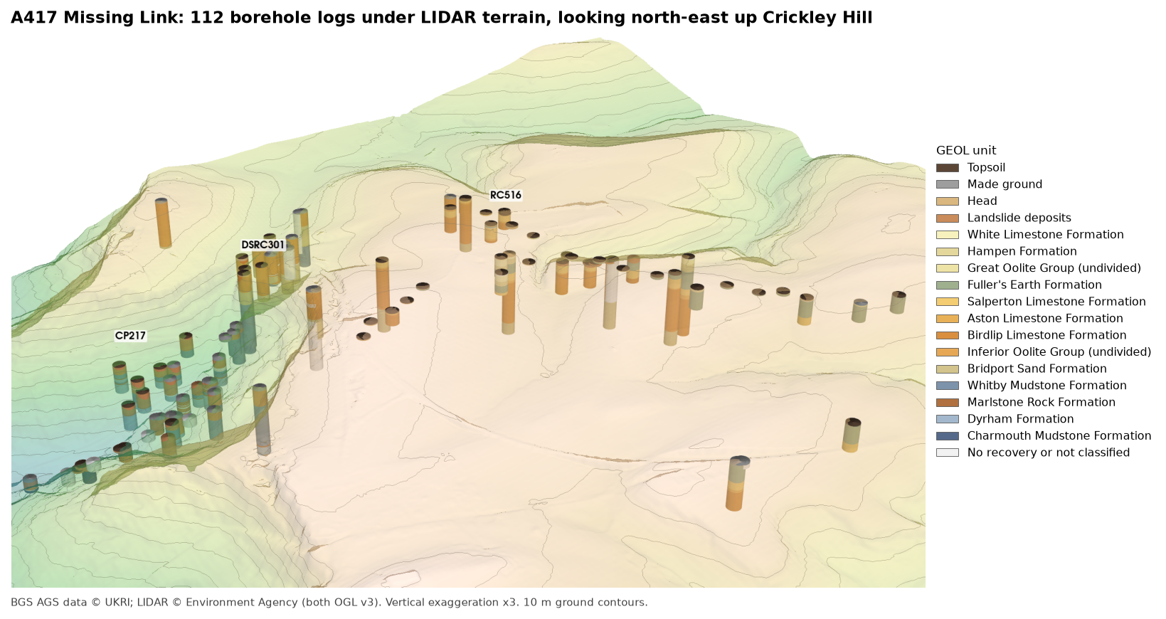
The terrain goes in semi-transparent with 10 m contours, then the logs, then a few labels. add_mesh(..., scalars="rgb", rgb=True) tells PyVista to use the stored colours directly:
pl = pv.Plotter(off_screen=True, window_size=(1800, 1150))pl.add_mesh(terrain, scalars="elevation", cmap="gist_earth", clim=[60, 330], opacity=0.4, smooth_shading=True, specular=0.0, ambient=0.3, show_scalar_bar=False)pl.add_mesh(terrain.contour(np.arange(90, 310, 10) * VE, scalars=terrain.points[:, 2]), color="#6f6a5f", line_width=1, opacity=0.5)pl.add_mesh(logs, scalars="rgb", rgb=True, smooth_shading=True, ambient=0.35)PyVista’s own legend tints its text, so compose() places the screenshot beside a matplotlib legend instead, with the data credit underneath. The result is the figure at the top of this post. Change off_screen=True to False and call pl.show() to get a window you can turn with the mouse.
Reading the overview from the vale (left) up to the plateau (right), the holes on the lower slopes are mostly blue-grey Lias mudstone under brown landslide deposits; on the escarpment they are orange Inferior Oolite limestone over pale Bridport Sand; and on the plateau they are green Fuller’s Earth and pale Great Oolite limestones. The tops of the cylinders follow the terrain closely, which is Part 2’s ground-level check seen in 3D.
Step 5: do neighbouring logs agree?
A good test of any set of logs is whether neighbouring holes agree about a surface they all pass through. The base of the Inferior Oolite is ideal: a hard limestone on top of a soft sand, which no driller is likely to miss. For every hole that logs Inferior Oolite limestone resting on Bridport Sand, the script finds the contact:
for lid, g in geol[rank > 0].groupby("LOCA_ID", sort=False): bds = g[g.UNIT == "BDS"] if bds.empty: continue b = bds.iloc[0] above = g[(g.UNIT.isin(["SALS", "ASLS", "BLPL", "IOG"])) & (g.GEOL_TOP < b.GEOL_TOP)] if above.empty: continue contacts.append(dict(LOCA_ID=lid, E=b.LOCA_NATE, N=b.LOCA_NATN, GL=b.LOCA_GL, depth=b.GEOL_TOP, z=b.top_mOD, above=above.iloc[-1].GEOL_DESC, below=b.GEOL_DESC))=== Step 5: do neighbouring logs agree? The base of the Inferior Oolite ===22 holes log Inferior Oolite limestone resting on Bridport Sand; the contact lies at 190.1 to 234.1 m ODfirst Bridport Sand material below the contact: {'CLAY': 9, 'MUDSTONE': 9, 'SILT': 3, 'SILTSTONE': 1}The material described just below the contact is clay, mudstone, silt or siltstone in every hole: the fine-grained top of the Bridport Sand, which here is much less sandy than its name suggests. The loggers were consistent about where the limestone stops.
Then we compare every pair of contact holes within 100 m of each other:
26 pairs of holes within 100 m of each other; 10 agree within 3 m a b metres_apart dz agree_3mDSRC404 DSRC419 6 0.3 TrueDSRC303 RC509 17 15.2 FalseDSRC302 RC508 23 13.7 FalseDSRC406 RC509 29 14.7 FalseDSRC303 DSRC406 36 0.4 TrueDSRC303 RC508 38 11.2 FalseDSRC109 DSRC301 41 0.3 True...Only 10 of 26 close pairs agree within 3 m, which at first looks poor. But the disagreements all involve the same three holes. DSRC404 and DSRC419, 6 m apart, agree to 0.3 m; DSRC303 and RC509, 17 m apart, differ by 15.2 m. Comparing each hole with the median of its neighbours picks out the three:
contact minus the median of its neighbours within 100 m (holes with 2+ neighbours):RC509 -15.2RC507 -13.9RC508 -11.2DSRCOH304 -4.0DSRC406 -0.4DSRC303 0.2DSRC325 2.0DSRC110 5.8DSRC109 6.3DSRC302 6.4DSRC301 6.8offset by more than 8 m: RC507, RC508, RC509. Without them, 12 pairs agree to within 6.3 m (median 1.1 m)Leave out RC507, RC508 and RC509 and the remaining 12 pairs agree to a median of 1.1 m. The three holes record the base of the limestone 11 to 15 m lower than the holes around them. Laid out side by side at true elevation, the difference is plain:
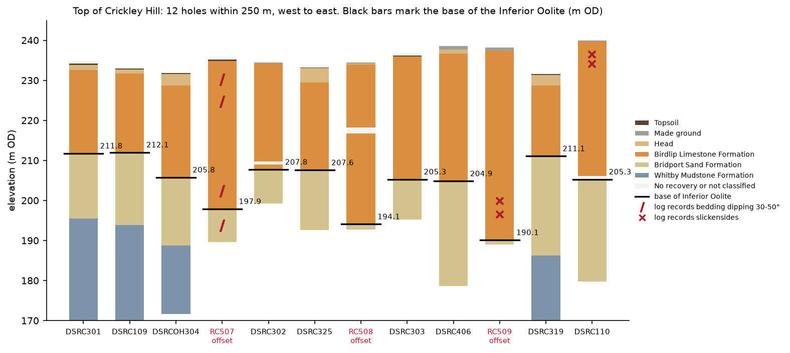
The ground surface over the three holes is no lower than over their neighbours, so the limestone in them is thicker: 47 m in RC509 against 31 m in DSRC303, 17 m away. The logs say why. The script searches the descriptions for the two things a logger notes when ground has moved: steeply dipping bedding and slickensides.
steep = geol.GEOL_DESC.str.extract(r"bedded \((\d+)\s*-\s*(\d+)\s*deg\)", expand=True).astype(float)geol["bedding_dip"] = steep[1]geol["slickensides"] = geol.GEOL_DESC.str.contains("slickensid", case=False)12 holes reach the contact within 250 m of the close-up centre; their logs record: DSRC110 2.95- 4.00 m Birdlip Limestone Formation slickensides DSRC110 5.30- 6.60 m Birdlip Limestone Formation slickensides RC507 1.60- 8.20 m Birdlip Limestone Formation bedding dipping up to 50 deg RC507 9.70- 11.20 m Birdlip Limestone Formation bedding dipping up to 50 deg RC507 28.36- 37.30 m Birdlip Limestone Formation bedding dipping up to 50 deg RC507 37.30- 45.60 m Bridport Sand Formation bedding dipping up to 50 deg RC509 36.40- 40.20 m Birdlip Limestone Formation slickensides RC509 40.20- 43.20 m Birdlip Limestone Formation slickensidesThe Cotswold limestones are close to horizontal, dipping a degree or two to the south-east. RC507 records bedding dipping at up to 50° from near the surface down into the Bridport Sand. RC509 records slickensides between 36.4 and 43.2 m, in the lower part of its limestone and 5 to 12 m above its contact. Of the nine holes that agree with each other, only DSRC110 records anything similar, slickensides between 3 and 7 m, and its contact is in line with its neighbours.
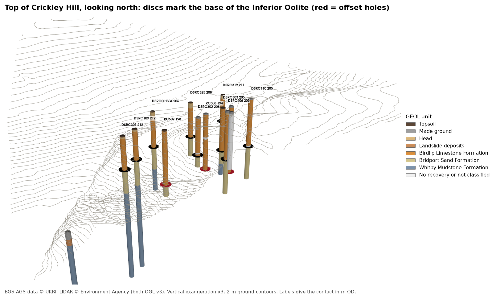
Put together, the evidence describes a block of limestone at the crest of the escarpment that has dropped 11 to 15 m relative to the ground around it, with its bedding tilted and slip surfaces within it. That is what cambering and valley-side foundering produce: at the edge of the Cotswold escarpment, the hard limestone cap slowly sags over the soft Bridport Sand and Lias mudstone beneath it, and blocks near the edge tilt and drop. A small fault would also lower a block, but would not usually tilt its bedding to 50°. Cross-sections drawn through these holes are the natural next test, and that is where Part 4 of the series starts.
Step 6: the same logs in the QGIS 3D map view
QGIS can draw borehole logs in 3D too. The script writes each interval as a vertical LineStringZ from its top to its base in British National Grid and m OD, along with the collars as 3D points and the contacts from Step 5:
lines = gpd.GeoDataFrame( {"LOCA_ID": geol.LOCA_ID, "unit": geol.UNIT, "unit_name": geol.UNIT.map(A.UNITS.name), "colour": geol.UNIT.map(A.UNITS.colour), "top_depth": geol.GEOL_TOP, "base_depth": geol.GEOL_BASE, "top_mOD": geol.top_mOD.round(2), "base_mOD": geol.base_mOD.round(2), "GEOL_DESC": geol.GEOL_DESC}, geometry=[LineString([(r.LOCA_NATE, r.LOCA_NATN, r.top_mOD), (r.LOCA_NATE, r.LOCA_NATN, r.base_mOD)]) for r in geol.itertuples()], crs="EPSG:27700")=== Step 6: write LineStringZ intervals for QGIS ===wrote output/a417_logs_3d.gpkg: 'intervals' 1564 LineStrings with z: True, 'collars' 112 points, 'base_inferior_oolite' 22 pointsterrain for QGIS 3D: a417_dtm_5m.tifqgis_3d_logs.py then builds a QGIS project around them with PyQGIS. Run it with the Python that comes with QGIS, as in Part 2:
"C:\Program Files\QGIS 3.40.12\bin\python-qgis-ltr.bat" qgis_3d_logs.pyA borehole log in 3D is only useful if you can see where it is, so the script puts the logs in the ground they came from. It does four things.
It cuts the terrain away in front of the logs. Borehole logs are underground, so a plain 3D view hides them inside the hill. The script copies the 5 m DTM and sets the ground south of a stepped cut line to no data: along the foot of the escarpment at northing 215700, then up to the crest at 215975. It then stands a vertical face along the cut, from 100 m OD up to the ground, so the cut reads as a solid block. QGIS meshes its 3D terrain in square tiles, coarsely, and a cut that wanders across them comes out ragged. A cut along tile edges stays straight, which is why the line is stepped rather than following the holes.
SECTION = [(391700.0, 215700.0), (393075.0, 215700.0), (393075.0, 215975.0), (393900.0, 215975.0)]
def south_of_cut(x, y, lip=0.0):    """True where the ground is cut away; lip moves the cut that far into the cut-away side."""    (_, y_foot), (x_step, _), (_, y_crest), _ = SECTION    return ((x < x_step + lip) & (y < y_foot - lip)) | ((x >= x_step + lip) & (y < y_crest - lip))
z[south_of_cut(xx, yy, lip=CUT_LIP) | ~np.isfinite(z)] = -9999
It moves the nearby holes onto the face. Every hole within 60 m of the cut is moved square onto it, 6 m in front, and each GEOL interval becomes a 16 m wide prism from its base to its top. The real holes are 0.1 to 0.2 m across, but at 2 km a true-width log would vanish. The offset_m field records how far each hole was moved.
It colours each prism by its unit, with one rule per unit and absolute altitude clamping, so each prism stays at its own height in m OD rather than being draped on the terrain. Height and extrusion come from the data, both multiplied by the same twofold vertical exaggeration as the terrain:
def extruded(colour: str) -> QgsPolygon3DSymbol:    sym = QgsPolygon3DSymbol()    sym.setAltitudeClamping(Qgis.AltitudeClamping.Absolute)    props = sym.dataDefinedProperties()    props.setProperty(QgsAbstract3DSymbol.Property.Height, QgsProperty.fromExpression(f'"base_mOD" * {EXAGGERATION}'))    props.setProperty(QgsAbstract3DSymbol.Property.ExtrusionHeight,                      QgsProperty.fromExpression(f'"thickness" * {EXAGGERATION}'))    sym.setDataDefinedProperties(props)    sym.setMaterialSettings(phong(colour))    return sym
root = QgsRuleBased3DRenderer.Rule(None)for u, (name, colour) in units.items():    root.appendChild(QgsRuleBased3DRenderer.Rule(extruded(colour), f"\"unit\" = '{u}'", name))columns.setRenderer3D(QgsRuleBased3DRenderer(root))
It drapes a map on the terrain. The ground is textured with OpenStreetMap under the LIDAR hillshade, so you can pick out the A417, the Crickley Hill country park and The Scrubbs. QGIS 3D can drape a live web map, but it is slow and the view can stall while the tiles load, so the script renders the two layers once, at 1 m per pixel, to a local GeoTIFF and drapes that instead:
ms = QgsMapSettings()ms.setDestinationCrs(QgsCoordinateReferenceSystem("EPSG:27700"))ms.setExtent(QgsRectangle(*VIEW_EXTENT))ms.setOutputSize(QSize(w, h)) # 1 m per pixelms.setLayers([hillshade, osm]) # the hillshade multiplies over the mapjob = QgsMapRendererSequentialJob(ms)job.start()job.waitForFinished()QGIS 3.40.12-Bratislavaintervals valid=True (1564) | dtm valid=Truehillshade valid=True | cutaway valid=True | osm valid=True | texture valid=Truecolumns: 450 prisms in 26 holes within 60 m of the section, radius 8 m | cut face: 501 strips from 100 m OD to groundholes on the section: CP102, CP104, CP104A, CP105, CP106, CP200, CP202, CP206, CP216, CP230, CPT202, DSRC107, DSRC108, DSRC109, DSRC301, DSRC302, DSRC406, OH405, RC507, RC508, RC509, TP201, TP204, TP205, TP207, TP601saved output/a417_logs_3d.qgz: 18 3D rules (TOPS, SLIP, CHAM, MGR, NR, DYS, WHM, MRB, HEAD, BLPL, BDS, HMB, FE, SALS, ASLS, WHL, IOG, GOG), terrain LIDAR DTM, cut awayOpen output/a417_logs_3d.qgz in QGIS Desktop and choose View > 3D Map Views > New 3D Map View. Then, in the Python console, run setup_3d_view(iface.mapCanvases3D()[0].mapSettings()) from the bottom of the script. It shows only the logs and the face, uses the cutaway DTM with the draped texture as terrain at twofold exaggeration, and sets the lighting. Turn the view to look north-east up the hill:
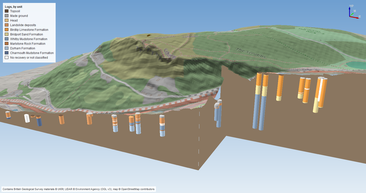
The crest holes show the escarpment’s layer cake: Birdlip Limestone at the top, then Bridport Sand, then Whitby Mudstone, with the contacts at much the same height from hole to hole. Down on the lower face the holes are short and mostly landslide deposits over Lias mudstone, which is the ground that has slipped off the scarp. That is the same story as the PyVista overview, but now in an ordinary QGIS project, alongside your other layers, where anyone can turn it round without writing code.
Frequently asked questions
How do I plot borehole logs in 3D in Python?
Join GEOL to LOCA on LOCA_ID, subtract each interval’s top and base depths from LOCA_GL to get elevations, and draw a cylinder or tube for each interval at the hole’s easting and northing. With PyVista, pv.Cylinder for each interval merged with pv.merge gives one fast mesh. Colour it by unit through a per-face RGB array.
Can QGIS show boreholes in 3D?
Yes. Store each interval as a polygon at the hole’s position with its base elevation and thickness as fields, then give the layer a 3D polygon symbol with absolute altitude clamping, the base as its height and the thickness as its extrusion. A rule-based 3D renderer gives each unit its own colour. Cutting the terrain away in front of the holes lets you see them below ground.
Why use vertical exaggeration?
The A417 holes are spread over 4 km but are at most 105 m deep, so at true scale they would look like pins. Three times exaggeration makes the layers visible while keeping the shape of the ground recognisable. Always say what exaggeration a figure uses.
What is cambering?
At the edge of an escarpment where hard rock caps softer clay or sand, the soft beds slowly squeeze out towards the valley and the cap rock sags over them. Blocks of the cap tilt and drop, and open fissures called gulls can form between them. It is common along the Cotswold escarpment and matters for foundations and cuttings.
Can I do this with any AGS file?
Yes. Steps 1 to 4 and 6 only need LOCA and GEOL. Swap the unit table in a417_ags.py for the formations on your site, and change the contact in Step 5 to a surface that most of your holes pass through.
Next steps
- Part 4: a geological cross-section draws a section along a line of boreholes, with ground level from LIDAR, which cuts straight through RC507 to RC509. After that come interpolated stratum surfaces such as rockhead (Part 5), test results such as SPT N-values (Part 6), and a 3D-printed ground model (Part 7).
- 3D terrain visualisation with PyVista goes further with PyVista terrain, lighting and camera control.
- Kriging spatial interpolation in Python introduces the interpolation methods that turn contacts like Step 5’s into continuous surfaces.
- Back to Part 1: Reading and validating AGS4 files or Part 2: Boreholes on a map.
Data and licences
- A417 Missing Link ground investigation (BGS deposited data item 173984; client Highways England, now National Highways; contractor Geotechnical Engineering Ltd), downloaded through the BGS AGS borehole index and export APIs. Contains British Geological Survey materials © UKRI 2026, licensed under the Open Government Licence v3.0.
- Environment Agency LIDAR Composite DTM 1 m, requested at 5 m from the Defra Data Services Platform WCS. © Environment Agency copyright and/or database right, licensed under the Open Government Licence v3.0. It is the terrain in every PyVista view and in the QGIS 3D view, and each figure carries the credit.
- OpenStreetMap, draped on the terrain in the QGIS 3D view. Map data © OpenStreetMap contributors, available under the Open Database Licence; the figure carries the credit.
- Code:
borehole_logs_3d.py,qgis_3d_logs.pyanda417_ags.py, tested with Python 3.12.0, python-ags4 1.2.0, PyVista 0.49.2, VTK 9.7.2, GeoPandas 1.2.0, rasterio 1.5.2, shapely 2.2.0 and QGIS 3.40.12.
Key terms
- Vertical exaggeration
- Stretching heights relative to horizontal distances so that thin layers and gentle slopes can be seen. All 3D views here use three times.
- Inferior Oolite
- A Middle Jurassic group of limestones that forms the steep face and crest of the Cotswold escarpment. Here it is the Salperton, Aston and Birdlip Limestone formations.
- Slickensides
- Polished, striated surfaces in rock or clay formed where one side has slid past the other. A logger records them because they show the ground has moved.
- Cambering
- The slow outward and downward sagging of a hard cap rock, such as the Cotswold limestones, over softer beds beneath it at the edge of a valley or escarpment. Blocks of cap rock tilt and drop, often opening fissures called gulls.
- LineStringZ
- A line whose vertices have x, y and z coordinates. A vertical one with the same x and y at both ends can represent one interval of a borehole log.
Data for this tutorial
- BGS AGS borehole data · Donated AGS ground investigation data, Open Government Licence
Licences and formats for each source are listed in the GIS data sources catalogue.