3D terrain visualisation in Python with PyVista: Helvellyn from LIDAR, Sentinel-2 and a GPX route

Short answer: to show terrain in 3D in Python, load the DEM as a NumPy array, build a PyVista StructuredGrid from the cell-centre coordinates and the heights (multiplied by a vertical exaggeration), give it texture coordinates, and render it with an image draped on top:

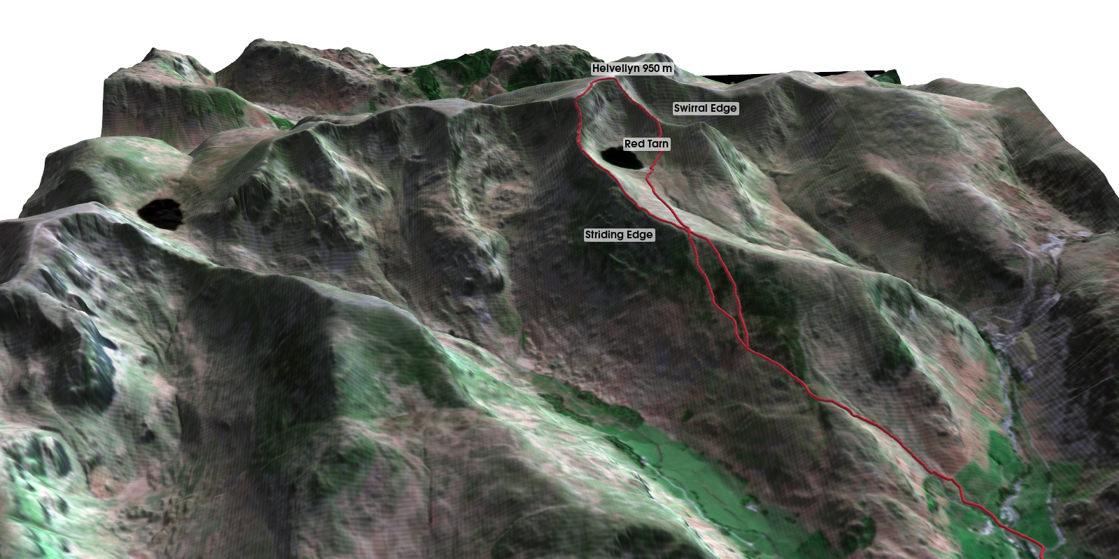
import pyvista as pv
pv.OFF_SCREEN = True                                    # no window needed, on Windows too
grid = pv.StructuredGrid(x, y, dem * 1.5)               # x, y: 2D arrays of cell centres
grid.texture_map_to_plane(origin=(0, 0, 0), point_u=(width, 0, 0), point_v=(0, height, 0), inplace=True)
pl = pv.Plotter(off_screen=True, window_size=(1600, 950))
pl.add_mesh(grid, texture=pv.Texture(rgb), smooth_shading=True)   # rgb: image on the same grid as the DEM
pl.screenshot("terrain.png")

The rest of this tutorial does this properly for a real place: Helvellyn in the Lake District, from the Environment Agency’s 1 m LIDAR, with a Sentinel-2 image and the classic walk from Glenridding over Striding Edge and back by Swirral Edge.

You will learn how to:

1. Download a LIDAR DTM from the Environment Agency WCS and mosaic it in NumPy.
2. Find a cloud-free Sentinel-2 day with STAC and reproject it onto the DEM grid.
3. Build a walking route from OpenStreetMap, write it to GPX, and read it back with gpxpy.
4. Turn the DEM into a PyVista StructuredGrid and check what each vertex is.
5. Align the texture correctly, and measure the error if you do not.
6. Compare vertical exaggerations and lighting set-ups.
7. Drape the GPX route, render a final scene off-screen and make a rotating MP4.

If you want a physical model instead of an image, the same DEM goes to a 3D printer in DEM to STL in Python. For an earlier take on a single track in 3D, see visualising a cycle track in 3D.

Set-up

py -3.12 -m venv .venv-terrain3d
.venv-terrain3d\Scripts\activate
pip install -r requirements.txt
python terrain_3d_pyvista.py

PyVista ships with VTK wheels for Windows, macOS and Linux, so there is nothing else to install. pv.OFF_SCREEN = True makes every plotter render to an image buffer. On Windows and macOS that works as is, with the normal graphics driver. A headless Linux server has no display, so install xvfb and run the script under xvfb-run, or install the EGL build of VTK.

The study area is a 9 × 7.5 km box in British National Grid (EPSG:27700) from 331000 to 340000 E and 511000 to 518500 N. That takes in Helvellyn, Red Tarn, Glenridding and the southern end of Ullswater.

Step 1: the LIDAR DTM from the Environment Agency WCS

The Environment Agency publishes its LIDAR Composite DTM at 1 m for almost all of England. The Defra Web Coverage Service will cut out any box and resample it on the server, so we ask for 1.5 km tiles at SCALEFACTOR=0.2, which gives 5 m cells:

X0, Y0, X1, Y1 = 331_000, 511_000, 340_000, 518_500   # 9 km x 7.5 km around Helvellyn, British National Grid
RES = 5.0
TILE = 1500
WCS = ("https://environment.data.gov.uk/spatialdata/lidar-composite-digital-terrain-model-dtm-1m/wcs"
       "?service=WCS&version=2.0.1&request=GetCoverage&format=image/tiff"
       "&CoverageId=13787b9a-26a4-4775-8523-806d13af58fc__Lidar_Composite_Elevation_DTM_1m")

H, W = int((Y1 - Y0) / RES), int((X1 - X0) / RES)
dem = np.full((H, W), np.nan)
for x in range(X0, X1, TILE):
    for y in range(Y0, Y1, TILE):
        tif = get(f"{WCS}&subset=E({x},{x + TILE})&subset=N({y},{y + TILE})&SCALEFACTOR={1 / RES}",
                  DATA / f"ea_dtm_{x}_{y}_{RES:.0f}m.tif")
        with rasterio.open(tif) as src:          # tiles share the 5 m grid: paste each in place
            a = src.read(1).astype("float64")
            a[a < -1000] = np.nan                 # no-data is -3.4e38
            r, c = int((Y1 - src.bounds.top) / RES), int((src.bounds.left - X0) / RES)
            dem[r:r + a.shape[0], c:c + a.shape[1]] = a

Every tile sits exactly on the same 5 m lattice, so pasting each one by its row and column offset is simpler and safer than a general mosaic. (With rasterio 1.5, rasterio.merge returned an array of zeros for these tiles, because of the very large negative no-data value.)

30 WCS tiles -> grid 1800 x 1500 cells of 5 m (9.0 x 7.5 km), origin 331000 E, 518500 N
no-data cells: 0 (0.00%), filled from the nearest valid cell
elevation 144.9 to 949.0 m (relief 804 m) | slope median 20.7 deg, 95th percentile 42.3 deg, max 82.1 deg

The relief is 804 m over 9 km and half the area is steeper than 20.7°: this is real mountain country, and that is why the exaggeration question in Step 6 matters. For hillshade, slope and aspect in more depth, see terrain analysis with rasterio.

Step 2: a clear Sentinel-2 day, reprojected onto the DEM grid

The Lake District is cloudy, so we search the Planetary Computer STAC for every summer Sentinel-2 Level-2A scene since May 2024 with under 20% cloud for the whole tile, and then check the cloud over our box using the scene classification layer (SCL). The box straddles the boundary between MGRS tiles T30UVF and T30UWF at 3° W, so each day is a mosaic of two tiles:

for day in sorted(by_day, key=lambda d: max(i.properties["eo:cloud_cover"] for i in by_day[d]))[:10]:
    scl = np.zeros((H20, W20), "uint8")
    for item in cat.search(collections=["sentinel-2-l2a"], bbox=bbox, datetime=f"{day}").items():
        with rasterio.open(item.assets["SCL"].href) as src:
            part = np.zeros_like(scl)
            reproject(rasterio.band(src, 1), part, dst_transform=from_origin(X0, Y1, 20, 20),
                      dst_crs="EPSG:27700", resampling=Resampling.nearest, src_nodata=0, dst_nodata=0)
        scl = np.where(scl == 0, part, scl)
    bad = np.isin(scl, [0, 3, 8, 9, 10]).mean() * 100     # no data, cloud shadow, cloud, cirrus

Then the red, green and blue bands of the chosen day are reprojected with rasterio.warp.reproject straight onto the DEM’s 5 m grid, so the image and the heights share one transform:

for b, band in enumerate(["B04", "B03", "B02"]):
    for item in day_items:
        with rasterio.open(item.assets[band].href) as src:
            part = np.zeros((H, W), "float32")
            reproject(rasterio.band(src, 1), part, dst_transform=dem_tf, dst_crs="EPSG:27700",
                      resampling=Resampling.bilinear, src_nodata=0, dst_nodata=0)
            rgb_bng[b] = np.where(rgb_bng[b] == 0, part, rgb_bng[b])

87 scenes with under 20% tile cloud; 25 summer days. The study area straddles MGRS tiles T30UVF, T30UWF, so each day is mosaicked
  2025-05-16: cloud, shadow or no data over the study area  0.60%
  2025-05-13: cloud, shadow or no data over the study area  0.00%
chosen: 13 May 2025, tiles S2C_MSIL2A_20250513T112131_R037_T30UWF_20250513T135636, S2C_MSIL2A_20250513T112131_R037_T30UVF_20250513T135636; 0.00% cloud or shadow over the study area
reprojected to the DEM grid: 1800 x 1500 cells of 5 m, empty cells 0.00% | the same area in EPSG:32630 (UTM 30N): 911 x 763 pixels of 10 m

The tile-level cloud figure is not enough on its own: a tile with 5% cloud can have all of it over the fells. For a wider treatment of SCL and other masks, see Sentinel-2 cloud masking in Python.

Step 3: a GPX route from OpenStreetMap

Most people bring their own GPX file from a watch or an app. To keep this reproducible, the script builds one. It reads the footpaths in the box from the Geofabrik Cumbria extract with pyosmium, makes a NetworkX graph, and chains shortest paths through the ends of the OSM ways named Striding Edge and Swirral Edge. The result is written to GPX with gpxpy, and everything after that works from the GPX file, exactly as it would with your own track:

track = gpxpy.parse((OUT / "helvellyn_route.gpx").read_text())
pts = np.array([(p.longitude, p.latitude) for p in track.tracks[0].segments[0].points])
rx, ry = to_bng.transform(pts[:, 0], pts[:, 1])
d = np.r_[0, np.cumsum(np.hypot(np.diff(rx), np.diff(ry)))]
step = np.arange(0, d[-1], RES)                        # densify to one point per DEM cell
rx, ry = np.interp(step, d, rx), np.interp(step, d, ry)


def sample(z, x, y):
    """Bilinear DEM height at BNG coordinates."""
    col, row = (x - X0) / RES - 0.5, (Y1 - y) / RES - 0.5
    return ndimage.map_coordinates(z, [row, col], order=1, mode="nearest")


rz = sample(dem, rx, ry)

Densifying to one point every 5 m matters. GPX points from OSM are only placed at bends, sometimes 100 m apart, and a straight line between them in 3D would cut through ridges and hang over corries.

walkable OSM network: 16,092 nodes, 16,345 segments; named ways found: Swirral Edge, Striding Edge
GPX: 683 track points written and read back; densified to 2,237 points every 5 m
route length 11.18 km | lowest 156 m, highest 949 m | total ascent 894 m (5-point smoothed LIDAR profile)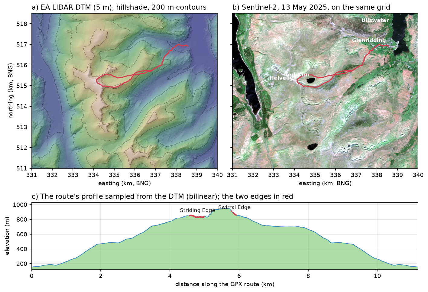

Step 4: from DEM to a PyVista StructuredGrid

A raster is already a structured mesh: every cell centre becomes one vertex, and neighbouring cells become quads. PyVista only needs three 2D arrays of the same shape for x, y and z:

cx, cy = np.meshgrid(X0 + RES * (np.arange(W) + 0.5), Y1 - RES * (np.arange(H) + 0.5))


def terrain(z, exag, stride=1, r0=0, c0=0):
    """StructuredGrid in local metres (origin at the SW corner) with texture coordinates.
    r0, c0: row and column offset when z is a window of the full DEM."""
    zz = z[::stride, ::stride]
    rows, cols = slice(r0, r0 + z.shape[0], stride), slice(c0, c0 + z.shape[1], stride)
    xs, ys = cx[rows, cols] - X0, cy[rows, cols] - Y0
    g = pv.StructuredGrid(xs, ys, zz * exag)
    g.texture_map_to_plane(origin=(0, 0, 0), point_u=(X1 - X0, 0, 0), point_v=(0, Y1 - Y0, 0), inplace=True)
    g["elevation"] = zz.ravel(order="F")
    return g


grid = terrain(dem_vis, EXAG)

Three details are worth copying:

• Local coordinates. Subtracting the south-west corner keeps x and y below 10,000. Raw BNG eastings and northings in the hundreds of thousands lose precision in the 32-bit floats that the graphics card uses, and the surface starts to shimmer.
• Texture coordinates from the box, not the mesh. texture_map_to_plane with an explicit origin and the full width and height gives u = 0 on the west edge and 1 on the east edge, and v = 0 at the south and 1 at the north. pv.Texture(rgb) maps image row 0 to v = 1, so a north-up array goes on the right way round with no flip.
• Scalars in Fortran order. A StructuredGrid built from 2D arrays stores points column by column, so per-point data must be raveled with order="F" to line up.

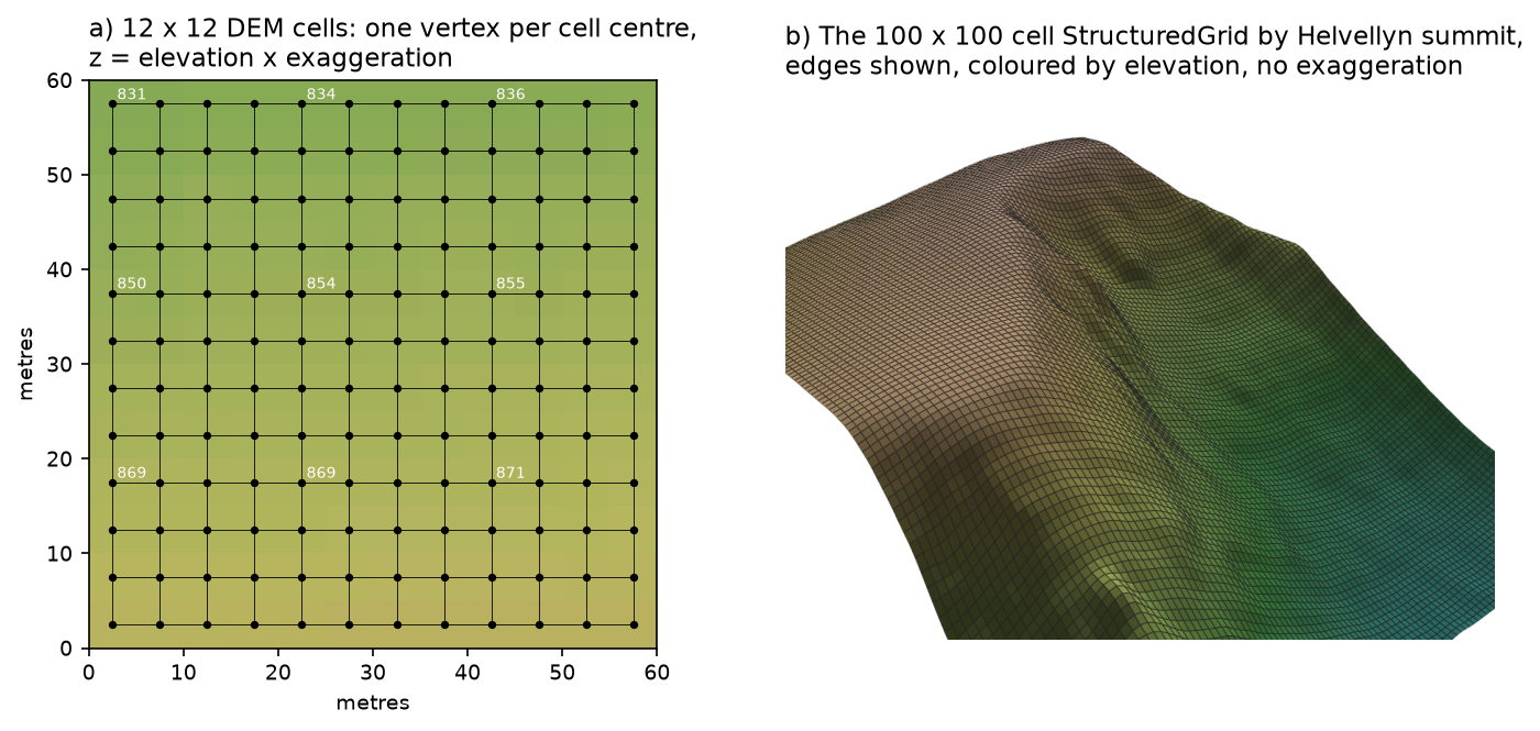
display DEM: Gaussian sigma 1 cell, mean absolute change 0.37 m, 95th percentile 1.12 m
StructuredGrid: dimensions (1500, 1800, 1), 2,700,000 points, 2,696,701 quad cells, 103 MiB
texture coordinates: u 0.000-1.000, v 0.000-1.000
as triangles: 5,393,402 triangles

The dem_vis array is the DTM with a one-cell Gaussian blur. The WCS resamples the 1 m LIDAR to 5 m by interpolation rather than averaging, so some 1 m micro-relief leaks through. Lit at screen resolution, that noise turns into a moiré of fine stripes. The blur changes the heights by 0.37 m on average and is used for the 3D meshes only; slopes, profiles and the route all use the unblurred DTM.

At 2.7 million points the full grid is 103 MiB. That is fine on a laptop GPU, but for the animation in Step 8 we take every second cell (stride=2), which quarters the size and looks the same at video resolution.

Step 5: texture alignment, done right

Sentinel-2 is delivered in UTM zone 30N. It is tempting to clip the image to the bounding box, resize it to the DEM’s shape and drape it. The script measures how far out that would be by transforming every DEM cell centre into UTM and comparing the true pixel with the pixel the naive resize would use:

ux, uy = Transformer.from_crs(27700, utm, always_xy=True).transform(cx, cy)
true_col, true_row = ~utm_tf * (ux, uy)
naive_col = (np.arange(W) + 0.5) / W * native.shape[2]
naive_row = (np.arange(H) + 0.5) / H * native.shape[1]
err = np.hypot(true_col - naive_col[None, :], true_row - naive_row[:, None]) * 10

naive resize vs proper reprojection: mean misplacement 65 m, max 130 m (UTM 30N grid north is rotated against BNG grid north)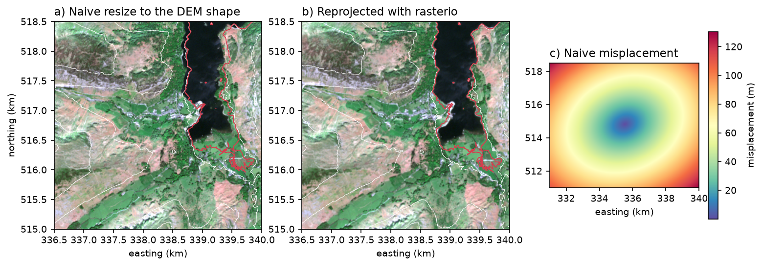

Sixty-five metres is thirteen DEM cells. On a 3D model it puts lakes on hillsides and fields on crags. The fix costs nothing: reproject the image onto the DEM’s grid, as in Step 2. The same applies to any pair of rasters in different projections; coordinate reference systems in Python covers the background.

Step 6: vertical exaggeration

The heights are multiplied by a factor before they go into the grid. That makes relief easier to read, but it also steepens every slope as drawn, to arctan(k · tan θ):

for ex in (1.0, 1.5, 3.0):
    g = terrain(dem_vis, ex)
    pl = plotter((900, 560))
    pl.add_mesh(g, texture=tex, ambient=0.25, diffuse=0.85, specular=0.0, smooth_shading=True)
    sun_light(pl); camera(pl, ex, az=100, el=24, dist=12_500)
    shots.append(pl.screenshot(return_img=True)); pl.close()

exaggeration 1.0x: z range in the scene 804 m against 9,000 m across; 95th percentile slope as drawn 42 deg
exaggeration 1.5x: z range in the scene 1,205 m against 9,000 m across; 95th percentile slope as drawn 54 deg
exaggeration 3.0x: z range in the scene 2,411 m against 9,000 m across; 95th percentile slope as drawn 70 deg

For a mountain area like this, 1× already shows the shape, and 1.5× brings out the corries and edges without making the Lake District look like the Alps. Flatter places need more: 3–5× for lowland river valleys, 10× or more for coastal plains. Whatever you choose, put it in the caption.

Step 7: lighting and hillshade

PyVista’s default light is attached to the camera, so the surface is lit from wherever you look at it and the relief goes flat. The script removes the default lights and adds one scene light from the north-west at 45°, the same direction as a conventional hillshade:

CENTRE = np.array([(X1 - X0) / 2, (Y1 - Y0) / 2, 0])
SUN = np.array([-0.5, 0.5, np.sqrt(0.5)])             # azimuth 315 (from the north-west), altitude 45 degrees


def sun_light(pl):
    pl.remove_all_lights()
    pl.add_light(pv.Light(position=tuple(CENTRE + SUN * 1e5), focal_point=tuple(CENTRE),
                          light_type="scene light", positional=False, intensity=1.0))

It then compares four set-ups. The third bakes a matplotlib LightSource hillshade into the image before draping it, shaded = rgb * (0.35 + 0.65 * hs), so that small features stay visible even on slopes that face the light.

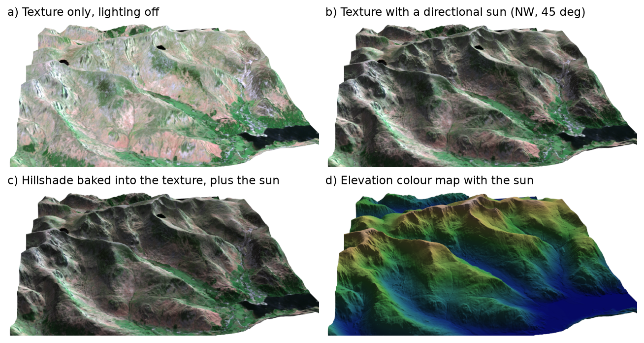
Option c is used for the final render. Option d is useful when the imagery is poor or the scene is too large for one image. Sentinel-2 water renders very dark in true colour, so Red Tarn and the lakes appear almost black; that is the real reflectance of deep, clear water at visible wavelengths.

Step 8: drape the GPX route and render the final scene

The route is a polyline at the DEM height plus 4 m, turned into a tube so it has a visible width from any angle:

LIFT = 4.0                                    # metres above the ground, so the line is not hidden in the mesh
line = pv.lines_from_points(np.c_[rx - X0, ry - Y0, (rz + LIFT) * EXAG])
tube = line.tube(radius=9)

pl = plotter((1600, 950))
pl.add_mesh(grid, texture=tex_shaded, ambient=0.35, diffuse=0.7, specular=0.0, smooth_shading=True)
pl.add_mesh(tube, color=RED, ambient=0.5, diffuse=0.6)
sun_light(pl)
pl.add_point_labels(lab_pts, list(labels), font_size=15, point_size=1, shape_opacity=0.65, shape_color="white",
                    text_color="black", always_visible=True, show_points=False)
camera(pl, EXAG, az=95, el=27, dist=8_200)
img = pl.screenshot(return_img=True, window_size=(1600, 950))

Remember to multiply the route heights by the same exaggeration as the terrain, or the line ends up underground on every slope. The camera helper places the camera on a compass bearing and elevation angle around the centre of the scene, which is easier to reason about than VTK’s raw position and focal point. The 1600 × 950 render, with smooth shading and anti-aliasing, takes 0.2 s.

Step 9: a rotating MP4

pl.open_movie uses imageio-ffmpeg to write a video, and pl.write_frame() adds the current view. Moving the camera bearing through 360° gives an orbit:

small = terrain(dem_vis, EXAG, stride=2)          # 10 m mesh: a quarter of the points, the same look at video size
pl = plotter((768, 432))
scene(pl, small, tex_shaded)
pl.open_movie(str(OUT / "helvellyn_orbit.mp4"), framerate=15, quality=5)
for i in range(120):
    camera(pl, EXAG, az=95 + 360 * i / 120, el=30, dist=11_000)
    pl.write_frame()
pl.close()

animation mesh: 675,000 points (every 2nd DEM cell)
[render 120 frames: 0.7 s]
helvellyn_orbit.mp4: 120 frames at 768 x 432, 8 s, 0.84 MB
helvellyn-orbit.html: 1.12 MB

Use a frame size divisible by 16 (768 × 432 rather than 800 × 450), or ffmpeg resizes the frames and warns. The script also writes the MP4 into a small HTML page as a data URI, which is what is embedded below:

For a truly interactive page, pl.export_html("scene.html") writes the whole scene with trame and vtk.js so readers can rotate it themselves. It needs the trame extras (pip install "pyvista[jupyter]"), and the file holds the full mesh and texture, so for a grid of millions of points it is many times larger than the 0.84 MB video. Decimate the mesh first (grid.extract_surface().triangulate().decimate(0.9)) if you go that way.

Limitations and honest caveats

• 5 m from the WCS, not 1 m. The server resamples by interpolation, and some 1 m micro-relief survives, so the 3D meshes use a 1-cell Gaussian blur (0.37 m mean change). For a full-resolution model of a small area, request SCALEFACTOR=1 and keep the box under about 2 × 2 km, or the mesh will exceed most GPUs’ memory.
• The image date is not the LIDAR date. The Sentinel-2 scene is from May 2025; the LIDAR composite mixes surveys from several years. Snow, felling and reservoir levels can disagree between the two.
• Sentinel-2 is 10 m. At 5 m terrain cells each image pixel spans four cells, so the texture looks soft in close-ups. Aerial photography at 25 cm is far sharper but is not openly licensed for England; some countries publish open orthophotos, such as the Netherlands through PDOK.
• The route comes from OSM geometry. Mapped paths can be tens of metres from the line people actually walk on rocky ground such as Striding Edge, and the ascent figure is sensitive to smoothing: 894 m on a 5-point smoothed LIDAR profile. A GPS track from a watch has its own noise, and a barometric altimeter measures the climb differently.
• Off-screen on Linux servers needs a virtual display (xvfb-run) or the EGL/OSMesa build of VTK. Windows and macOS need neither.
• Not a navigation aid. The edges are serious scrambles with long drops. Use an OS map and check the conditions before walking them.

Frequently asked questions

How do I make a 3D terrain map in Python?

Read the DEM into a NumPy array (with rasterio), build x and y arrays of the cell-centre coordinates with np.meshgrid, and pass them with the heights to pyvista.StructuredGrid(x, y, z). Add it to a pv.Plotter with a colour map or an image texture, set the camera and call screenshot(). Multiply the heights by a vertical exaggeration if the area is flat. Matplotlib’s plot_surface works for small grids, but it is slow above a few hundred thousand cells and cannot drape an image well.

How do I drape a satellite image on a DEM in PyVista?

First reproject the image onto exactly the same grid as the DEM with rasterio.warp.reproject, so that pixel (i, j) of the image sits over cell (i, j) of the DEM. Then give the mesh texture coordinates with texture_map_to_plane, using the DEM’s origin and full width and height, and pass texture=pv.Texture(rgb) to add_mesh. Do not just resize the image: here that misplaced it by 65 m on average.

What vertical exaggeration should I use for a DEM?

Use the smallest value that makes the landforms readable. Mountain areas such as the Lake District need 1–1.5×; rolling hills 2–3×; lowland valleys and coastal plains 5–10× or more. Remember that exaggeration steepens slopes as drawn: at 3× the 42° slopes here look like 70°. State the value in the caption.

Can PyVista render without a display on Windows?

Yes. Set pv.OFF_SCREEN = True or pass off_screen=True to pv.Plotter, and call screenshot() or write_frame(). On Windows and macOS this uses the normal graphics driver with no window and needs no xvfb. Only headless Linux servers need a virtual display or the EGL build of VTK.

How do I show a GPX track in 3D in Python?

Read it with gpxpy, transform the latitudes and longitudes into the DEM’s projected CRS with pyproj, densify the line to about one point per DEM cell, and sample the DEM height under each point with bilinear interpolation (scipy.ndimage.map_coordinates). Multiply by the same vertical exaggeration as the terrain, lift it a few metres, and draw it with pv.lines_from_points(...).tube(radius=...).

How do I export a PyVista scene to HTML or video?

For a video, call pl.open_movie("out.mp4"), move the camera, and call pl.write_frame() for each frame; imageio-ffmpeg does the encoding. For an interactive web page, pl.export_html("scene.html") writes the mesh and a vtk.js viewer into one file, which can be large for detailed terrain; decimate the mesh first.

Next steps

• 3D-print the same DEM with DEM to STL in Python, or in QGIS with creating a 3D-printed DEM.
• Revisit visualising a cycle track in 3D and swap its terrain for the PyVista scene here.
• Work out what can be seen from the summit with viewshed analysis in Python, and drape the visible area as a texture instead of the image.
• Go from the gridded DTM to the raw points with LIDAR point clouds in Python with laspy; PyVista renders point clouds with pv.PolyData(xyz).
• Compute slope, aspect and roughness to colour the surface with terrain analysis with rasterio.

Data and licences

• Elevation: Environment Agency, LIDAR Composite DTM 1 m, via the Defra Data Services Platform WCS. © Environment Agency copyright and/or database right 2026. All rights reserved. Licensed under the Open Government Licence v3.0.
• Imagery: Contains modified Copernicus Sentinel data 2025, Sentinel-2 Level-2A, accessed through the Microsoft Planetary Computer. Copernicus data are free and open under the Copernicus data licence.
• Paths: © OpenStreetMap contributors, available under the Open Database Licence. Cumbria extract from Geofabrik, downloaded on 3 November 2026.
• Code: terrain_3d_pyvista.py, tested with Python 3.12.0, pyvista 0.49.2, vtk 9.7.1, rasterio 1.5.2, numpy 2.5.4, pyproj 3.8.0, scipy 1.18.1, pystac-client 0.9.1, planetary-computer 1.0.0, osmium 4.3.2, networkx 3.7, gpxpy 1.6.2, imageio 2.38.1, imageio-ffmpeg 0.8.0 and matplotlib 3.11.2.