Rooftop solar potential from LiDAR in Python: pvlib, PVGIS and shading for every roof
Estimate rooftop solar potential in Python for 2,148 buildings in Manchester: take a 1 m Environment Agency LiDAR DSM and Overture Maps footprints, compute roof slope and aspect, trace horizon angles for shading from neighbours and trees, build a sun map from a PVGIS typical year with pvlib, check it against pvlib's Perez model and PVGIS, then estimate kWp and kWh per year per roof and rank the best roofs.
- Level
- Advanced
- Tested with
- Python 3.12
- Source code
- Download scripts
Key takeaways
- A 1 m LiDAR DSM, building footprints and one typical weather year are enough to estimate solar output for every roof. Here 2,148 buildings in Levenshulme, Manchester, take about a minute on a laptop.
- On an open 35° south-facing plane the sun-map model gives 1,026 kWh/m²/yr, matching pvlib's isotropic model exactly and within 6–8% of pvlib Perez (1,089) and PVGIS SARAH (1,109). It is deliberately conservative.
- Aspect matters far more than shading in a low-rise suburb: median south-facing pitches get 1,000 kWh/m²/yr against 711 for north-facing ones, while neighbours and trees remove only 2.8% of the beam.
- With stated assumptions (20% panels, 0.80 performance ratio, 70% coverage), the area could host 13.8 MWp and 10.1 GWh/yr, and 58% of house-sized roofs could cover a typical household's 2,700 kWh.
Before you start
- Comfort with numpy arrays and GeoPandas. Building footprints from LiDAR and terrain analysis with rasterio are good warm-ups
- Python 3.10+ with pvlib, h5py, duckdb, numpy, pandas, scipy, rasterio, pyproj, shapely, geopandas, pyogrio, requests and matplotlib
- An internet connection: LiDAR from the Environment Agency, footprints from Overture Maps and weather from PVGIS, all without an account
Short answer: to estimate rooftop solar potential in Python, you need three inputs: a LiDAR DSM (1 m or finer), building footprints and a weather file. First, mask the DSM to roof cells with the footprints and a height-above-ground threshold, and compute each cell’s slope and aspect. Next, trace horizon angles across the DSM so you know when neighbours, trees and chimneys shade it. Then, for each hour of a typical year (from PVGIS via pvlib.iotools.get_pvgis_tmy), use pvlib to find the sun’s position and add up the beam light that reaches the tilted roof when it is not shaded, plus diffuse and reflected light. Finally, convert kWh/m² to kWh per roof with explicit assumptions: panel efficiency, performance ratio and the share of the roof you can cover.
In this tutorial we do this for 2,148 buildings in Levenshulme, Manchester, a 1 km × 0.8 km block of Victorian terraces, semis, schools and shops, using Environment Agency LiDAR, Overture Maps footprints and PVGIS weather. We check the model against pvlib and PVGIS before trusting it.
You will learn how to:
- download a 1 m LiDAR DSM and DTM from the Environment Agency and building footprints from Overture Maps with DuckDB;
- find roof cells and compute slope and aspect with Horn’s method;
- compute horizon angles in 72 directions to model shading over the whole year;
- use pvlib with a PVGIS typical year to build a sun map, and check it against pvlib’s isotropic and Perez models, PVGIS SARAH and a clear-sky model;
- compute annual irradiation on 133,662 roof cells in under a second;
- turn irradiation into kWp and kWh per building, with stated assumptions, and rank the roofs.
All outputs below are real results from rooftop_solar.py, run on 23 October 2026 with Python 3.12.0, pvlib 0.16.1, rasterio 1.5.2, duckdb 2.0.0, geopandas 1.2.0 and numpy 2.5.4.
The assumptions, up front
A solar potential number is only as good as its assumptions. These are the ones in the script; change them at the top and re-run:
| Assumption | Value | Why |
|---|---|---|
| Panel efficiency | 20% | Typical 2026 monocrystalline modules are 20–22% at standard test conditions |
| Performance ratio | 0.80 | Losses in inverter, cabling, heat, dirt and mismatch; 0.75–0.85 is normal |
| Roof coverage | 70% | Edges, vents, skylights, access paths and fire setbacks |
| Usable roof cell | slope ≤ 60° and ≥ 800 kWh/m²/yr | Steeper cells are walls and dormers; below 800, panels rarely pay back in Manchester |
| Roof threshold | 2.5 m above the DTM | Separates roofs from cars, walls and garden furniture |
| Household demand | 2,700 kWh/yr | Ofgem’s typical domestic electricity consumption (medium) |
| Flat roofs | panels lie flat | No tilted racking, so a conservative yield |
These give a technical potential: what the roofs could produce. They ignore structural capacity, listed buildings, conservation areas, grid limits and cost.
Step 1: Environment Agency LiDAR DSM and DTM
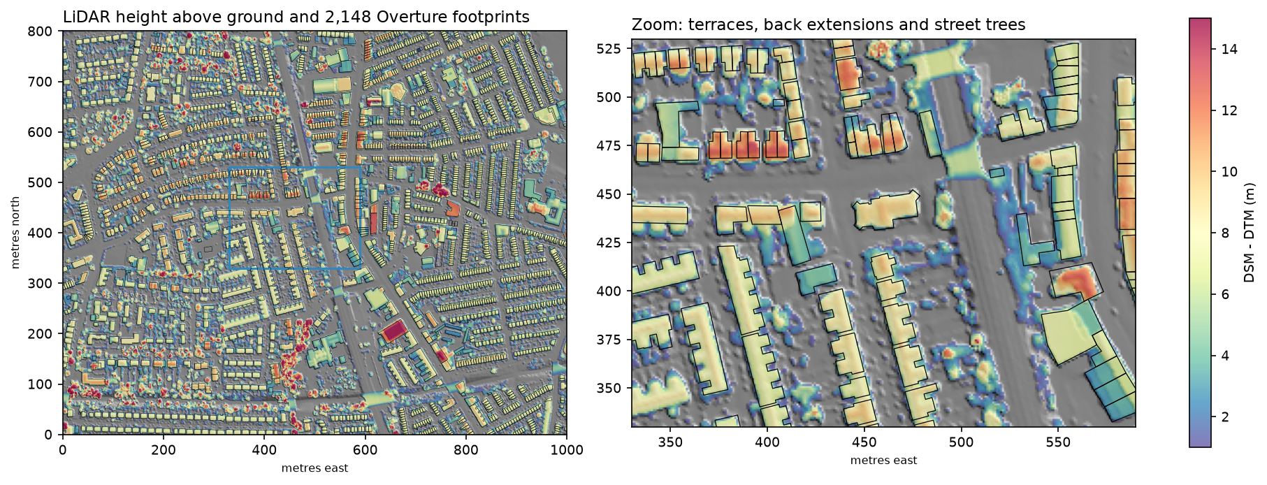
The Environment Agency publishes the LIDAR Composite for England at 1 m: a first-return DSM, which includes roofs and trees, and a bare-earth DTM. Both can be read through a WCS with no key, one tile at a time. We fetch 2 km × 2 km, larger than the 1 km × 0.8 km study area, so that shading from buildings and trees up to 300 m away is included:
AOI = (386800, 393700, 387800, 394500)        # xmin, ymin, xmax, ymax: 1 km x 0.8 km of roofs to assessFETCH = (386000, 393000, 388000, 395000)      # 2 km x 2 km of LiDAR, so shading from up to 300 m away is seen
def ea_wcs(product, x0, y0, size=1000):    """One 1 km x 1 km GeoTIFF from the Environment Agency WCS (no key needed)."""    service, cov = EA_WCS[product]    url = (f"https://environment.data.gov.uk/spatialdata/{service}/wcs?service=WCS&version=2.0.1"           f"&request=GetCoverage&CoverageId={cov}&format=image/tiff"           f"&subset=E({x0},{x0 + size})&subset=N({y0},{y0 + size})")    return requests.get(url, timeout=180).content   # the script adds retries and caches each tile
dsm, TF = ea_mosaic("dsm")dtm, _ = ea_mosaic("dtm")dsm = ndimage.median_filter(dsm, size=3) # knock down single-pixel LiDAR noise before taking slopesndsm = dsm - dtmgrid 2000 x 2000 cells of 1 m | no data: DSM 0.00%, DTM 0.00%DTM 37.5..61.8 m | DSM 37.5..82.7 m | cells over 2.5 m above ground: 31.4%The ground is nearly flat (37.5–61.8 m), so the shading comes from buildings and trees rather than hills. The 3 × 3 median filter matters: raw first-return LiDAR is noisy at the 10–20 cm level, which would make slopes on a 1 m grid jump around.
Step 2: Overture Maps building footprints with DuckDB
Overture Maps combines OpenStreetMap buildings with machine-learning footprints from Microsoft and others, as GeoParquet on S3. DuckDB can query just our bounding box. Overture’s STAC collections.parquet lists the bounding box of every file, so we read only the files that overlap:
release = requests.get("https://stac.overturemaps.org/catalog.json", timeout=60).json()["latest"]con = duckdb.connect()con.sql("INSTALL spatial; LOAD spatial; INSTALL httpfs; LOAD httpfs; SET s3_region = 'us-west-2';")overlaps = f"bbox.xmin <= {xmax} AND bbox.xmax >= {xmin} AND bbox.ymin <= {ymax} AND bbox.ymax >= {ymin}"files = [r[0] for r in con.sql(f""" SELECT assets.aws.alternate.s3.href FROM read_parquet('https://stac.overturemaps.org/{release}/collections.parquet') WHERE collection = 'building' AND {overlaps}""").fetchall()]df = con.sql(f""" SELECT id, subtype, class, height, num_floors, list_filter(sources, lambda s: s.property = '')[1].dataset AS source, ST_AsWKB(geometry) AS wkb FROM read_parquet({files}) WHERE {overlaps}""").df()We then rasterise the footprints to the 1 m grid, shrink each one by a cell (footprints and LiDAR never line up perfectly), and keep cells more than 2.5 m above the DTM:
bid = rasterize(((g, i + 1) for i, g in enumerate(bld.geometry)), out_shape=(H, W), transform=ATF, fill=0, dtype="int32")inner = ndimage.binary_erosion(bid > 0, iterations=1)roof = inner & (ndsm[A] > MIN_HEIGHT)AOI centre 53.4435 N, 2.1927 W | query bbox -2.2012, 53.4389, -2.1842, 53.4481Overture release 2026-10-21.0: 3,274 buildings in the query boxbuildings with a centroid in the AOI: 2,148 | sources: OpenStreetMap 1,903, Microsoft ML Buildings 245footprint area: median 56 m2, total 18.8 ha (24% of the AOI)footprint cells over 2.5 m in the nDSM: 92.7% | roof cells after a 1-cell inward buffer: 133,66292.7% of footprint cells are more than 2.5 m above the ground in the LiDAR, which is a good sign that the two datasets agree. The other 7% are low outbuildings, footprint edges that spill onto the pavement, and buildings built or demolished since the LiDAR was flown.
Step 3: roof slope and aspect
Slope and aspect come from the DSM’s gradients. Horn’s method, the one GDAL and most GIS packages use, takes the weighted differences of the eight neighbours of each cell:
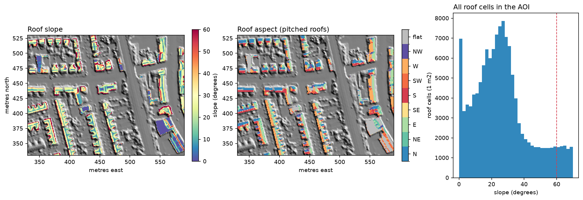
def horn(z, res=1.0): """Slope (degrees) and aspect (degrees clockwise from north, the direction the slope faces).""" p = np.pad(z, 1, mode="edge") a, b, c = p[:-2, :-2], p[:-2, 1:-1], p[:-2, 2:] d, f = p[1:-1, :-2], p[1:-1, 2:] g, h, i = p[2:, :-2], p[2:, 1:-1], p[2:, 2:] dzdx = ((c + 2 * f + i) - (a + 2 * d + g)) / (8 * res) # rise towards the east dzdy = ((a + 2 * b + c) - (g + 2 * h + i)) / (8 * res) # rise towards the north slope = np.degrees(np.arctan(np.hypot(dzdx, dzdy))) aspect = (np.degrees(np.arctan2(-dzdx, -dzdy)) + 360) % 360 # downslope direction return slope, aspectroof cells: flat (<10 deg) 16.3% | pitched 10-60 deg 74.7% | steeper 9.0%pitched roof slope: median 26 deg, interquartile 19-34 degpitched roof cells by the way they face: N 18%, NE 10%, E 16%, SE 9%, S 17%, SW 9%, W 14%, NW 8%Three-quarters of roof cells are pitched. The aspects cluster on the four cardinal directions because the streets run on a grid. A median slope of 26° is lower than the 35–40° typical of Victorian terraces. This is a known effect of 1 m LiDAR: cells on ridges, valleys and eaves average two planes or a roof and the ground, which pulls slopes down. Fitting planes to the point cloud per roof face would do better.
Step 4: horizon angles for shading
A roof is shaded when an obstacle in the sun’s direction rises above the sun. So for every roof cell we compute the horizon angle in 72 directions, every 5°. We march outwards along each direction, from 2 m to 300 m, and keep the steepest angle up to the DSM. Vectorising over all roof cells at once keeps this fast:
AZ = np.arange(2.5, 360, 5.0)                  # 72 horizon directions, clockwise from northSTEPS = np.r_[np.arange(2, 30, 1), np.arange(30, 100, 2), np.arange(100, 301, 5)]  # ray-march distances (m)NOISE = 0.3             # m; LiDAR noise allowance so a rough roof does not shade itself
for k, az in enumerate(AZ): best = np.zeros(len(rr), "float32") sa, ca = np.sin(np.radians(az)), np.cos(np.radians(az)) for d in STEPS: off = -int(round(d * ca)) * WF + int(round(d * sa)) np.maximum(best, (zf[flat_idx + off] - z0 - NOISE) / d, out=best) hor[k] = np.degrees(np.arctan(best))72 directions x 104 steps (2-300 m) for 133,662 roof cells in 8.0 srelative sky view: median 1.00, 10th percentile 0.95The same horizons give a relative sky view factor: the share of the sky a tilted roof cell can see, compared with the same plane with nothing around it. Diffuse light is scaled by it. The median of 1.00 shows that most roofs in a two-storey suburb have an open sky; the worst 10% lose 5% or more.
The horizon idea is the same as a viewshed seen from the other side. For a full treatment of line of sight over a DEM, see viewshed analysis in Python.
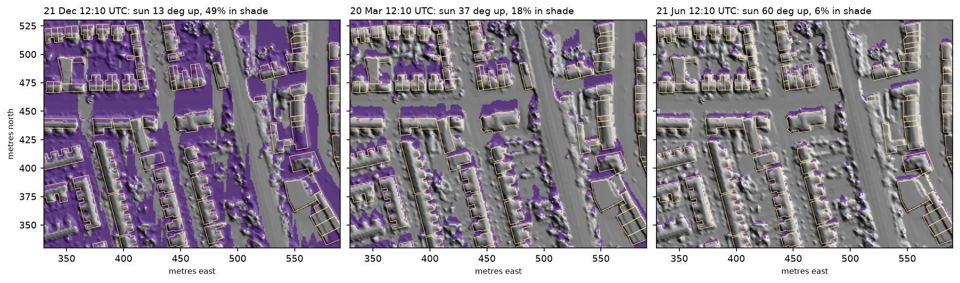
2026-12-21 12:10 UTC: sun elevation 13.2 deg, azimuth 181 deg, 49% of the zoom window in shadow2026-03-20 12:10 UTC: sun elevation 36.5 deg, azimuth 178 deg, 18% of the zoom window in shadow2026-06-21 12:10 UTC: sun elevation 60.0 deg, azimuth 180 deg, 6% of the zoom window in shadowStep 5: a PVGIS typical year and a sun map with pvlib
PVGIS (the European Commission’s Photovoltaic Geographical Information System) provides a typical meteorological year for any point in Europe, built from satellite irradiance. pvlib downloads it in one line. We switch PVGIS’s own horizon off (usehorizon=False), because our LiDAR horizons will do the shading.
Running every hour of the year through every roof cell would be slow. So we build a sun map: we group the 2,933 sunlit hours into sky cells of 5° in azimuth and 2° in elevation. In each cell we keep three sums of DNI that make the incidence angle on any plane a linear formula:
tmy, meta = pvlib.iotools.get_pvgis_tmy(LAT, LON, usehorizon=False, map_variables=True)times = tmy.index + pd.Timedelta(minutes=30)             # hourly values: put the sun in the middle of the hoursp = pvlib.solarposition.get_solarposition(times, LAT, LON)
sun = tmy[(tmy["elevation"] > 0) & (tmy["dni"] > 0)].copy()z = np.radians(sun["zenith"]); azr = np.radians(sun["azimuth"])sun["SA"] = sun["dni"] * np.cos(z)                       # Wh/m2 that a horizontal plane would getsun["SB"] = sun["dni"] * np.sin(z) * np.cos(azr)sun["SC"] = sun["dni"] * np.sin(z) * np.sin(azr)sun["az_bin"] = (sun["azimuth"] // 5).astype(int)sun["el_bin"] = (sun["elevation"] // 2).astype(int)sun["w_el"] = sun["dni"] * sun["elevation"]sunmap = sun.groupby(["az_bin", "el_bin"])[["SA", "SB", "SC", "dni", "w_el"]].sum().reset_index()sunmap["el"] = sunmap["w_el"] / sunmap["dni"]            # DNI-weighted sun elevation in the bin
For a plane with slope β and aspect γ, the beam energy from a sky cell is SA·cos β + sin β·(SB·cos γ + SC·sin γ), and it counts only when the sun is above the cell’s horizon in that direction. Diffuse light uses the isotropic sky, scaled by the sky view factor, and ground-reflected light uses an albedo of 0.2:
def annual_irradiance(slope_deg, aspect_deg, horizon_deg, svf): """Annual beam + diffuse + reflected irradiation (kWh/m2 of tilted surface).""" b, g = np.radians(slope_deg), np.radians(aspect_deg) cb, sb, cg, sg = np.cos(b), np.sin(b), np.cos(g), np.sin(g) beam = np.zeros(np.shape(slope_deg), "float64") for row in sunmap.itertuples(): inc = row.SA * cb + sb * (row.SB * cg + row.SC * sg) lit = horizon_deg[row.az_bin] < row.el beam += np.where(lit, np.maximum(inc, 0), 0) diffuse = tmy["dhi"].sum() * (1 + cb) / 2 * svf reflected = tmy["ghi"].sum() * ALBEDO * (1 - cb) / 2 return beam / 1000, diffuse / 1000, reflected / 1000TMY 8,760 hours | annual GHI 918 kWh/m2, DNI 740, DHI 572 | diffuse share of GHI 62%2,933 sunlit hours grouped into 463 sky cells (5 deg azimuth x 2 deg elevation) | beam on a horizontal plane 347 kWh/m2Manchester gets 918 kWh/m² a year on a horizontal surface, and 62% of it is diffuse. That is why north-facing roofs here still produce something, and why shading by neighbours matters less than in sunnier places.
Step 6: check the model on an open plane
Before applying the model to 133,662 cells, test it on a case with known answers: an unshaded plane tilted 35° and facing due south. We compare it with pvlib’s hourly transposition (isotropic and Perez), with ten years of PVGIS SARAH hourly data for the same plane, and with pvlib’s Ineichen clear-sky model as an upper bound:
poa = pvlib.irradiance.get_total_irradiance(35, 180, tmy["zenith"], tmy["azimuth"], dni_h, tmy["ghi"], tmy["dhi"], albedo=ALBEDO, model="isotropic")["poa_global"]poa_perez = pvlib.irradiance.get_total_irradiance(35, 180, tmy["zenith"], tmy["azimuth"], dni_h, tmy["ghi"], tmy["dhi"], dni_extra=dni_extra.values, albedo=ALBEDO, airmass=pvlib.atmosphere.get_relative_airmass(tmy["zenith"]).values, model="perez")["poa_global"]cs = pvlib.location.Location(LAT, LON).get_clearsky(times, model="ineichen")hourly, _ = pvlib.iotools.get_pvgis_hourly(LAT, LON, start=2014, end=2023, surface_tilt=35, surface_azimuth=180, components=True, usehorizon=False, pvcalculation=True, peakpower=1, loss=14)sun-map model (this script) : 1026 kWh/m2/yr (beam 489, diffuse 520, reflected 17)pvlib hourly, isotropic sky : 1026 kWh/m2/yrpvlib hourly, Perez sky : 1089 kWh/m2/yrPVGIS SARAH 2014-2023 mean : 1109 kWh/m2/yrpvlib Ineichen clear sky (no cloud): 1929 kWh/m2/yrspecific yield: ours 820 kWh/kWp (PR 0.8) | PVGIS PV model, 14% system loss 882 kWh/kWp| Method | kWh/m²/yr on 35° south |
|---|---|
| Sun-map model (this tutorial) | 1,026 |
| pvlib, isotropic sky | 1,026 |
| pvlib, Perez sky | 1,089 |
| PVGIS SARAH, 2014–2023 mean | 1,109 |
| Clear sky (Ineichen), no cloud | 1,929 |
The sun map reproduces pvlib’s hourly isotropic result exactly, so binning the sun into 463 sky cells loses nothing. The isotropic sky model is known to underestimate tilted surfaces, because it ignores the brighter sky around the sun and near the horizon. The Perez model and PVGIS are 6–8% higher. Our estimates are therefore conservative. Cloud halves the clear-sky potential in Manchester. Our specific yield of 820 kWh/kWp is 7% below PVGIS’s own PV model (882 kWh/kWp with 14% losses), which is within the range of real UK systems.
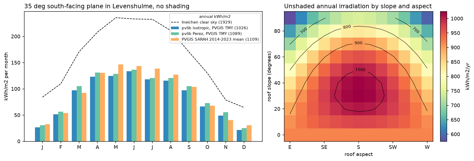
best unshaded orientation on the grid: slope 30 deg, aspect 180 deg, 1024 kWh/m2/yr | flat 919 | vertical south wall 746The heat map is a handy rule of thumb for Manchester: anything from south-east to south-west at 20–50° gets more than 950 kWh/m², within 7% of the best. East- and west-facing roofs at 30° still get about 850, only 7% less than a flat roof (919), and panels on a pitch shed dirt and water better than flat ones.
Step 7: annual irradiation on every roof cell
With the sun map and horizons in hand, the whole study area is one function call:
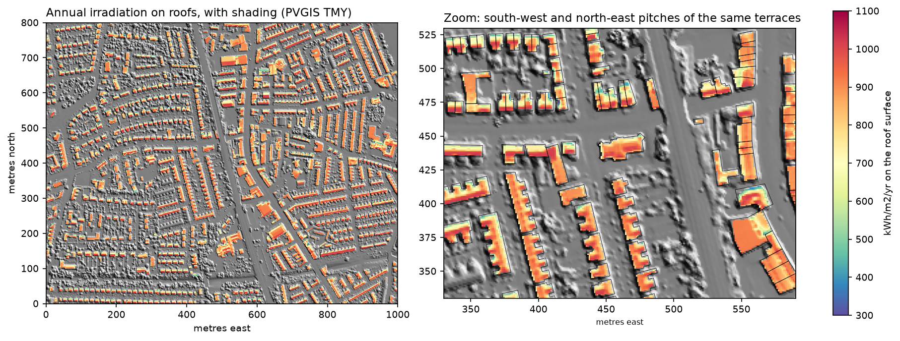
beam, diffuse, refl = annual_irradiance(s, a, hor, svf_rel)irr = beam + diffuse + refl463 sky cells x 133,662 roof cells in 0.2 sannual irradiation on roof cells: median 871 kWh/m2, 90th percentile 994, max 1026beam lost to shading from neighbours, trees and chimneys: 2.8% of the unshaded beammedian kWh/m2/yr on pitched roofs by aspect: N 711, NE 759, E 851, SE 962, S 1000, SW 943, W 870, NW 738 | flat roofs 908Shading removes only 2.8% of the beam across all roofs. In a suburb of two-storey houses, roofs are the highest surfaces around; shading matters much more for lower roofs, extensions and city centres. Aspect dominates instead: a south-facing pitch receives 41% more than a north-facing one (1,000 against 711 kWh/m²).
Step 8: kWh per building and the best roofs
Converting irradiation to energy needs the assumptions from the table above. A cell on a pitched roof has more surface than its 1 m² footprint (1/cos β), and only the usable cells count:
usable = (s <= MAX_SLOPE) & (irr >= MIN_IRR)tilted_m2 = 1 / np.cos(np.radians(s)) # a 1 m x 1 m cell on a 40 deg roof is 1.31 m2 of roofkwh = np.where(usable, irr * tilted_m2 * COVERAGE * PANEL_EFF * PERF_RATIO, 0)kwp = np.where(usable, tilted_m2 * COVERAGE * PANEL_EFF, 0) # 1 m2 at 20% = 0.2 kWp at 1000 W/m2We then sum the cells per building with a pandas groupby on the rasterised building ID:
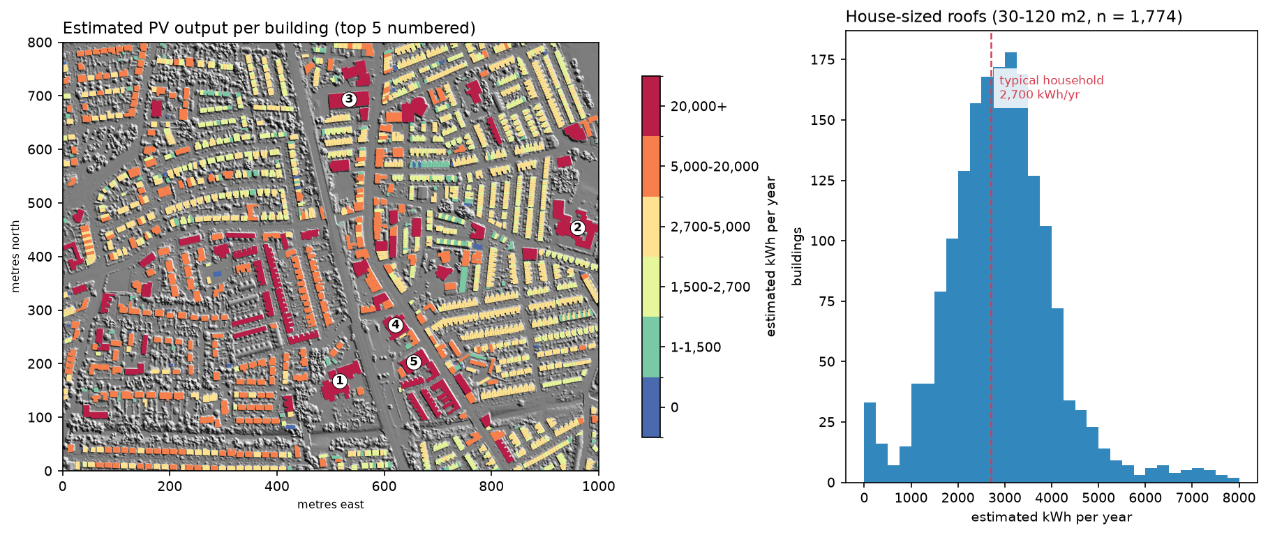
assumptions: efficiency 20%, performance ratio 0.8, coverage 70%, usable if slope <= 60 deg and >= 800 kWh/m2/yrusable share of roof area: 57%AOI total: 13.8 MWp, 10.1 GWh/yr = 3,748 typical households (2,700 kWh each)house-sized footprints (30-120 m2): 1,774 | median 3.9 kWp, 2,922 kWh/yr | 58% could cover 2,700 kWh/yr | 1% have no usable roof
top 10 roofs by annual output: rank       id       type  footprint_m2  usable_m2   kwp  kwh_yr  kwh_kwp  mean_irr    1 37d7b994     school          2763       1779 249.0  179598      721       902    2 0ca0beb5     school          2798       1621 226.9  164641      726       907    3 06f69560          -          1978       1537 215.2  154820      719       899    4 58398829          -          1402       1081 151.4  111407      736       920    5 923b7ea9 commercial          1347        978 137.0  100910      737       921    6 080a529b  religious          1479        871 121.9   86348      708       885    7 e21169e8     retail          1234        752 105.3   76383      725       907    8 9bc185f7     school           806        673  94.2   68492      727       909    9 917b5410    medical           782        590  82.5   59317      719       898   10 fef13b60      civic           853        560  78.4   56135      716       895
The typical house roof could take 3.9 kWp and produce 2,922 kWh a year, close to the 4 kWp systems commonly fitted in the UK. 58% of house-sized roofs could cover a typical household’s annual electricity use. That does not mean the house would be self-sufficient: most output comes in summer and in the middle of the day.
The top ten are schools, shops, a church, a surgery and a civic building. Large, mostly flat roofs are the obvious first targets for community or council schemes. Their yield of about 720 kWh/kWp is lower than a south pitch’s because the script assumes panels lie flat; tilting them at 10–15° on racks raises the yield per panel, but needs gaps between rows, so fewer panels fit. The full ranking is written to output/roof_ranking.csv, with Overture IDs you can join back to the footprints.
Pitfalls and limitations
- Roof planes from a raster. On a 1 m grid, ridges and eaves mix two planes, so slopes are biased low (median 26° here) and small roofs lose a large share of cells to the 1-cell buffer. Plane fitting on the classified point cloud, or a 25–50 cm DSM, does better.
- Obstructions smaller than the grid. Dormers, chimneys and roof windows a metre or two across are only partly resolved, and skylights and vents are not detected at all. The 70% coverage factor absorbs some of this.
- The LiDAR date. The DSM is a composite of surveys from different years. Trees grow, extensions are built and some roofs already have panels; check the survey dates in the Environment Agency’s metadata.
- Footprint quality. 245 of the footprints are machine-learning outlines from Microsoft, which are less precise than OpenStreetMap’s. Joined terraces may be one footprint per house or one per row.
- Isotropic diffuse light. The isotropic sky model underestimates tilted planes by 6–8% here compared with Perez and PVGIS. A Perez sun map, which needs a sky-brightness distribution per hour, would close most of the gap.
- Temperature and system design. A single performance ratio of 0.80 hides real differences between systems. For a single building, use pvlib’s ModelChain with a real module and inverter, or PVGIS’s PV calculator, with the roof’s slope, aspect and horizon from this tutorial.
- Technical, not economic, potential. Structural capacity, heritage protection, grid connections, prices and export tariffs decide what is actually built.
Frequently asked questions
How do you calculate rooftop solar potential in Python?
You need a DSM of the roofs (ideally LiDAR at 1 m or better), building footprints and hourly weather data. Compute slope and aspect for each roof cell, find when each cell is shaded by tracing horizon angles over the DSM, and add up beam, diffuse and reflected irradiance over a typical year with pvlib’s solar position and transposition functions. Then multiply the usable roof area by panel efficiency, a performance ratio and a coverage factor to get kWh per year.
What is pvlib used for?
pvlib is an open-source Python library for modelling photovoltaic systems. It computes solar position, clear-sky irradiance, the transposition of horizontal irradiance onto tilted planes (isotropic, Hay-Davies, Perez and others), cell temperature, module and inverter output, and whole-system yield with ModelChain. Its iotools module also downloads weather data from PVGIS, NSRDB and other services, as in this tutorial.
How much solar energy does a roof get in the UK?
In Manchester, an unshaded roof facing south at 30–35° receives about 1,025–1,110 kWh/m² a year, depending on the model; a flat roof gets about 920 and a north-facing pitch about 710. Southern England gets 10–20% more. A typical 4 kWp domestic system in Manchester produces roughly 3,000–3,500 kWh a year.
Can LiDAR be used for solar potential mapping?
Yes; it is the standard input for city-scale solar maps. A LiDAR DSM gives the slope and aspect of each roof plane and the height of everything that can cast a shadow on it, from neighbouring houses to trees. In England, the Environment Agency publishes a free 1 m DSM; the Netherlands (AHN), Denmark, Switzerland and many US states (USGS 3DEP) offer similar data.
What is the difference between PVGIS and pvlib?
PVGIS is a European Commission web service and database: it supplies satellite-derived irradiance and typical years for Europe, Africa and much of Asia, and runs a simple PV model on its servers. pvlib is a Python library that models PV systems on your machine from any weather data. They work well together: pvlib can download PVGIS data with pvlib.iotools.get_pvgis_tmy and get_pvgis_hourly.
Does shading from trees and neighbours matter much?
It depends on the setting. In this suburb of two-storey terraces, shading removed only 2.8% of the direct sunlight on roofs overall, because roofs are the highest surfaces around. It matters much more for single-storey extensions, roofs next to tall buildings or mature trees, and in dense city centres, and much more in winter: at noon on 21 December, half of our zoom window was in shadow.
Next steps
- Build the footprints and heights from the point cloud itself in building footprints and heights from LiDAR, and learn the point-cloud basics in LiDAR point clouds in Python with laspy.
- Compute slope, aspect and hillshade for terrain with raster terrain analysis in Python with rasterio.
- Query Overture buildings for a whole city with GeoParquet and DuckDB, then process them at scale with fast vector geoprocessing.
- Use the same DSM and horizon ideas for visibility in viewshed analysis in Python.
- Put the ranked roofs on a web map with Folium, or summarise them by ward with zonal statistics in Python.
- Compare with surface temperature in land surface temperature from Landsat in Python: roofs that get the most sun are often the hottest.
Data and licences
- LiDAR: Environment Agency LIDAR Composite first-return DSM and DTM, 1 m. © Environment Agency copyright and/or database right 2026. All rights reserved. Available under the Open Government Licence v3.0. Accessed from the Environment Agency WCS on 23 October 2026.
- Building footprints: Overture Maps Foundation, release 2026-10-21.0, buildings theme, under the Open Database Licence (ODbL). Includes © OpenStreetMap contributors and Microsoft ML Buildings. Accessed from Overture’s S3 bucket with DuckDB on 23 October 2026.
- Weather: PVGIS typical meteorological year and PVGIS-SARAH hourly data, 2014–2023, © European Union, Joint Research Centre. Free to reuse with attribution. Accessed through the PVGIS API with pvlib on 23 October 2026.
- Household consumption: Ofgem typical domestic consumption values (electricity, medium: 2,700 kWh a year).
- Code:
rooftop_solar.py, tested with Python 3.12.0, pvlib 0.16.1, h5py 3.16.0, duckdb 2.0.0, numpy 2.5.4, pandas 3.0.6, scipy 1.18.1, rasterio 1.5.2, pyproj 3.8.0, shapely 2.2.0, geopandas 1.2.0, pyogrio 0.13.0 and matplotlib 3.11.2.
Key terms
- Irradiation and irradiance
- Irradiance is solar power per square metre at an instant (W/m²); irradiation is energy over a period (kWh/m², here per year). Solar potential maps show irradiation.
- GHI, DNI and DHI
- Global horizontal, direct normal and diffuse horizontal irradiance: the three components a weather file gives. Beam light comes from the sun's disc; diffuse light from the rest of the sky.
- Plane of array (POA)
- Irradiance on the tilted surface of a panel or roof, computed from GHI, DNI and DHI with a transposition model such as isotropic or Perez.
- TMY
- Typical meteorological year: 12 real months picked from a long record to represent average conditions. PVGIS builds one from satellite data for any location in Europe.
- Performance ratio
- The share of the energy a panel would produce at its rated efficiency that actually reaches the grid, after losses in the inverter, cables, heat, dirt and mismatch. 0.75–0.85 is typical.
- Horizon angle
- The elevation angle of the highest obstacle seen from a point in a given direction. If the sun is below the horizon angle in its direction, the point is in shadow.
Data for this tutorial
- Environment Agency National LIDAR Programme · LIDAR Composite 1 m first-return DSM and DTM for England, via WCS
- Overture Maps · Building footprints (OpenStreetMap and Microsoft ML), queried with DuckDB
- PVGIS (European Commission JRC) · Typical meteorological year and hourly SARAH irradiance, via pvlib.iotools
Licences and formats for each source are listed in the GIS data sources catalogue.