Extract building footprints and heights from LiDAR in Python (USGS 3DEP, downtown Madison)
Turn classified LiDAR into building footprints with heights in Python: stream USGS 3DEP COPC tiles, build a DTM and a building nDSM from ASPRS class 6 points, polygonise and regularise the mask, split roofs at height steps, compute height statistics per building, score the result against OpenStreetMap with IoU, and export a GeoPackage and a 3D view.
- Level
- Intermediate
- Tested with
- Python 3.12
- Source code
- Download scripts
Key takeaways
- If the lidar is already classified, the building points (ASPRS class 6) do most of the work: a building nDSM above 2.5 m, a little morphology and rasterio's shapes() give footprints in a few seconds.
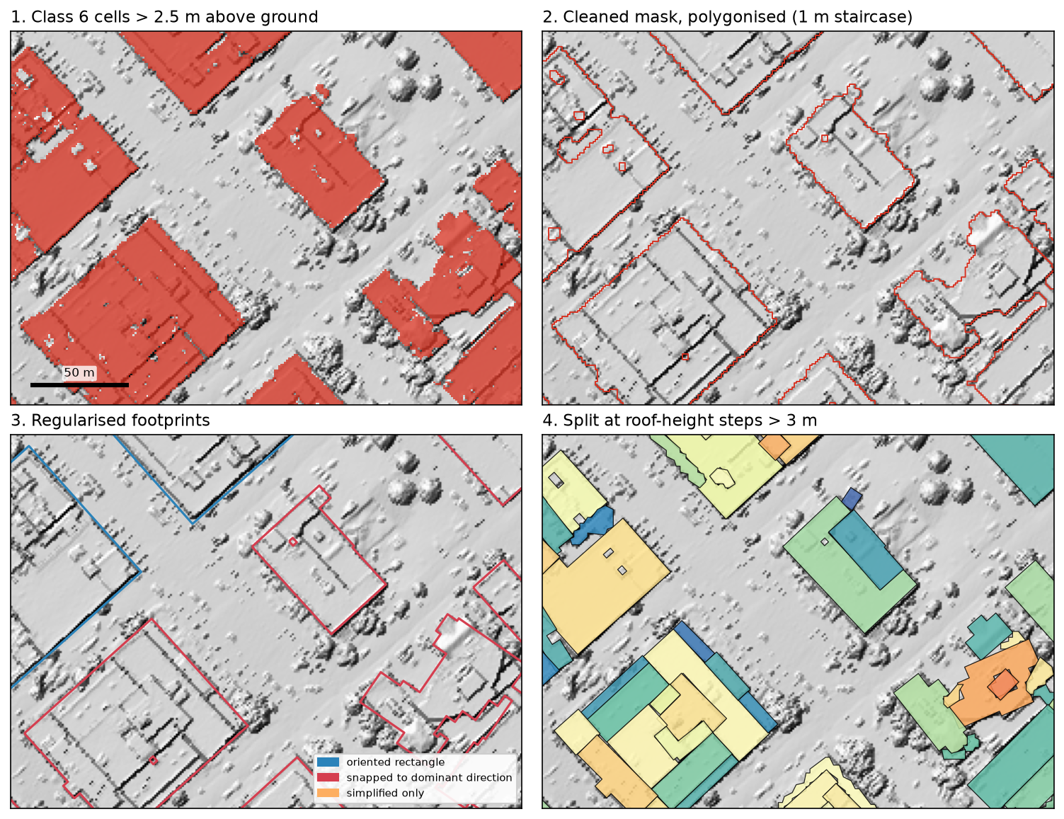
- Raw raster outlines have 1 m staircase edges (136 vertices per building on average). Rotating each building to its dominant direction and snapping edges orthogonally cut that to 16 vertices, at a median IoU of 0.889 with the staircase.
- Heights come from the points, not the raster. The highest return on the Wisconsin State Capitol is 86.3 m above the DTM, 0.4 m below its official 86.7 m.
- Against OpenStreetMap, the lidar footprints agree at a pixel IoU of 0.789 (precision 0.857, recall 0.909), but only 46.6% match one OSM building one-to-one, because lidar sees joined terraces and blocks as one roof.
Before you start
- Work through LiDAR point clouds in Python with laspy first: it covers COPC, ASPRS classes, the DTM and the DSM
- Python 3.10+ with laspy[lazrs], numpy, scipy, pandas, rasterio, pyproj, shapely, geopandas, osmnx, pystac-client, planetary-computer and matplotlib
- An internet connection: the lidar is streamed from the Microsoft Planetary Computer with no account or API key
Short answer: to extract building footprints from LiDAR in Python, keep the points classified as buildings (ASPRS class 6), grid them to a 1 m raster and subtract a ground DTM to get a building nDSM. Then threshold it (here at 2.5 m above ground), clean the mask with a morphological closing and opening, and turn each connected region into a polygon with rasterio.features.shapes. Finally, regularise the 1 m staircase outlines into straight, perpendicular edges. For building height, take the class 6 points inside each polygon and report the median, 95th percentile and maximum height above the DTM. If your point cloud has no building class, you need a classifier first (PDAL, lidR or a deep-learning model). Everything after the mask stays the same.
In this tutorial we do the whole job on 1 km² of downtown Madison, Wisconsin, around the State Capitol, with free USGS 3DEP lidar. We check the footprints against OpenStreetMap and the Capitol’s published height, and export a GeoPackage you can open in QGIS.
You will learn how to:
- find and stream only the points you need from USGS 3DEP Cloud Optimised Point Clouds;
- build a DTM from ground points and a building nDSM from class 6 points;
- turn the building mask into footprint polygons, and split joined buildings where the roof height jumps;
- regularise the outlines with oriented rectangles and orthogonal edge snapping;
- compute height statistics per building from the points and check them against a known height;
- score the footprints against OpenStreetMap with pixel and object IoU;
- export a GeoPackage, a GeoTIFF and a CSV, and draw a 3D extrusion with matplotlib.
All outputs below are real results from building_footprints.py, run on 14 October 2026 with Python 3.12, laspy 2.7.0, rasterio 1.5.2, shapely 2.2.0, geopandas 1.2.0 and osmnx 2.1.1.
Why extract buildings from a point cloud?
Footprints are easy to find: OpenStreetMap, Microsoft, Google and Overture all publish them. Heights are not. Only 5 of the 601 OSM buildings in our area have a height tag. Airborne lidar measures every roof directly, to about 10 cm vertically, so it is the usual source for 3D city models, solar potential, flood exposure, urban heat studies and checking building data.
Lidar also gives you an independent footprint. Comparing it with an existing layer shows missing buildings, demolitions and badly drawn outlines.
Step 1: stream classified lidar for the area of interest
USGS 3DEP publishes most of the United States as COPC files on the Microsoft Planetary Computer. Not every 3DEP project classifies buildings; many deliver only ground and unclassified points. The WI 4-County Statewide 2017 project does use class 6, which is why we picked Madison.
We search the STAC catalogue with a box of 1 km × 1 km around the Capitol and read only the points inside it:
LON, LAT = -89.38440, 43.07470   # Wisconsin State Capitol dome, MadisonEPSG = 26916                      # NAD83 / UTM zone 16N, the CRS of this lidar projectHALF = 500                        # 1 km x 1 km area of interestRES = 1.0                         # grid cell size in metres
catalog = pystac_client.Client.open("https://planetarycomputer.microsoft.com/api/stac/v1",                                    modifier=planetary_computer.sign_inplace)items = list(catalog.search(collections=["3dep-lidar-copc"], bbox=[lon0, lat0, lon1, lat1]).items())items = [it for it in items if "WI_4CountyStatewide_2017" in it.id]
bounds = laspy.Bounds(mins=np.array([xmin, ymin]), maxs=np.array([xmax, ymax]))for it in items:    with laspy.CopcReader.open(it.assets["data"].href) as reader:        pts = reader.query(bounds)          # only the octree nodes inside the box are downloaded
The script merges the parts into one LAZ file and caches it, so later runs start immediately:
USGS_LPC_WI_4CountyStatewide_2017_A17_0922  points=4,838,400USGS_LPC_WI_4CountyStatewide_2017_A17_0872  points=8,367,037USGS_LPC_WI_4CountyStatewide_2017_A17_0871  points=6,874,459
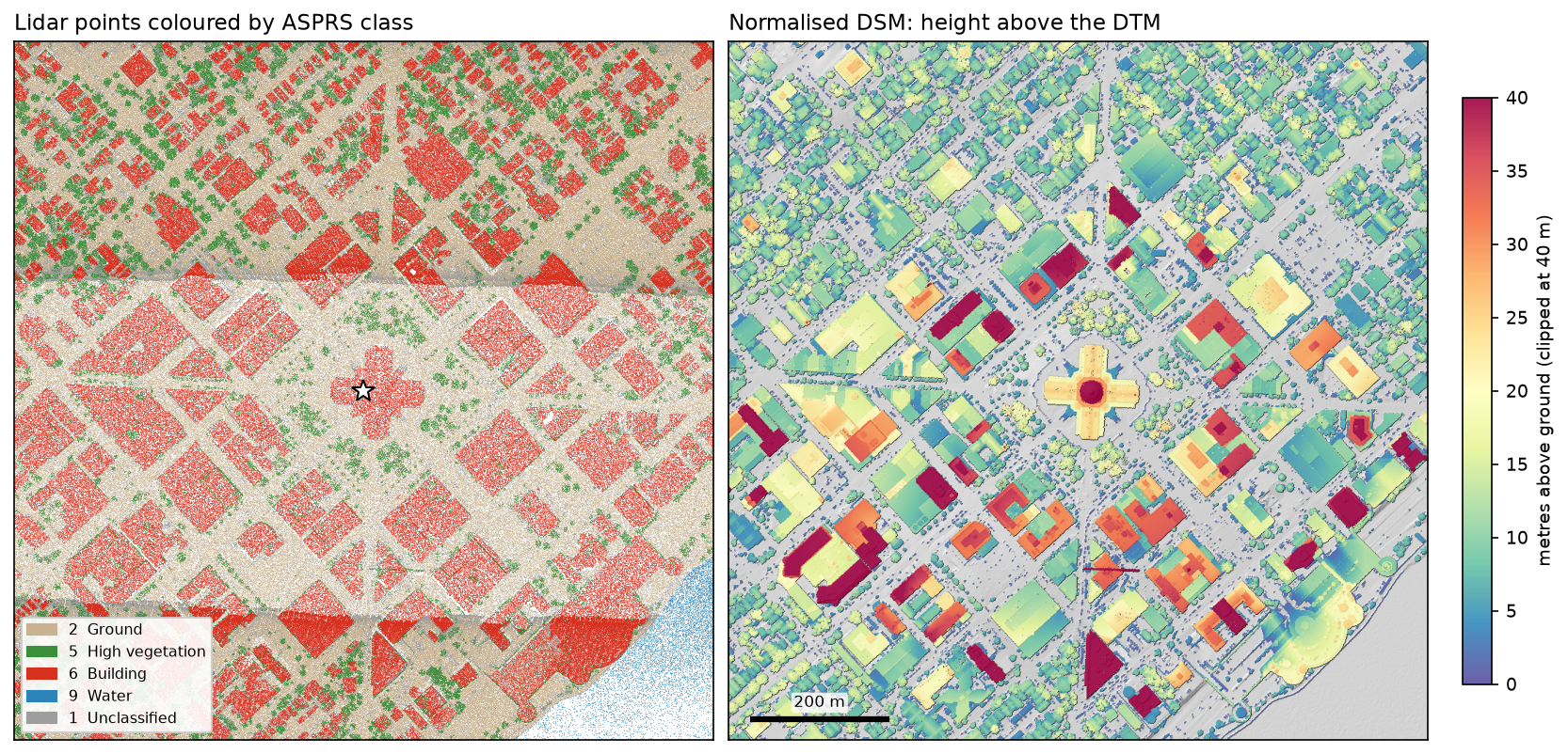
CRS: NAD83 / UTM zone 16N + NAVD88 heightpoints: 5,134,845 | density 5.1 points/m²class     points   share   name    1    432,774    8.4%   Unclassified    2  2,327,880   45.3%   Ground    5    865,795   16.9%   High vegetation    6  1,474,900   28.7%   Building    7      1,075    0.0%   Low noise    9     31,027    0.6%   Water   10        253    0.0%   Rail   17        494    0.0%   Bridge deck   18        647    0.0%   High noise
Three tiles hold 20 million points, but we only download the 5.1 million inside our square. 28.7% of them are building points, which is typical for a city centre.
Step 2: build a DTM and a building nDSM
A footprint is defined by height above the ground, not above sea level, so we need a bare-earth DTM first. We grid ground (class 2) and water (class 9) returns to 1 m and interpolate under the buildings, where there are no ground points. Then we take the highest class 6 return in each cell and subtract the DTM:
ground = grid_mean(np.isin(cls, [2, 9]))known = np.isfinite(ground)rr, cc = np.nonzero(known)gr, gc = np.nonzero(~known)filled = griddata((rr, cc), ground[known], (gr, gc), method="linear")nearest = griddata((rr, cc), ground[known], (gr, gc), method="nearest")dtm = ground.copy()dtm[gr, gc] = np.where(np.isfinite(filled), filled, nearest)
bld_top = grid_max(cls == 6) # highest building return per 1 m cellndsm_bld = bld_top - dtmDTM cells with a ground or water return: 60.4%DTM 245.6..284.0 m | building nDSM max 86.3 mOnly 60% of cells have a ground return; the other 40% are under roofs and trees. Linear interpolation across a building is fine here because downtown Madison is fairly flat, but on steep ground it can put the DTM a few metres too high or low under large buildings.
Step 3: from building points to a clean mask
A cell is a building if its highest class 6 return is more than 2.5 m above the DTM. Lower class 6 returns are mostly walls, steps and misclassified points. At 5 points/m², some 1 m cells inside a roof get no return at all, so we close small gaps, fill holes smaller than 9 m², open the mask to remove thin slivers and drop anything under 20 m²:
MIN_HEIGHT = 2.5 # metres above ground: lower class 6 cells are walls, steps or misclassified pointsMIN_AREA = 20 # m²: drop garden sheds and stray clustersraw = np.isfinite(ndsm_bld) & (ndsm_bld > MIN_HEIGHT)mask = ndimage.binary_closing(raw, structure=np.ones((3, 3)), iterations=1)holes = ndimage.binary_fill_holes(mask) & ~maskhole_lab, _ = ndimage.label(holes)small = np.nonzero(np.bincount(hole_lab.ravel()) < 9)[0]mask |= np.isin(hole_lab, small[small > 0])mask = ndimage.binary_opening(mask, structure=np.ones((2, 2)))labels, n = ndimage.label(mask)cells with a class 6 return > 2.5 m above ground: 360,203 (36.0%)after closing, hole filling and opening: 371,854 cells, 251 connected footprints of 20 m² or moreSplit joined buildings at roof-height steps
Downtown blocks are often built wall to wall, so one connected region can contain several buildings. Lidar cannot see a party wall, but it can see a step in roof height. Where the height changes by more than 3 m within one cell, we cut the region, label the pieces, and give the wall cells to the nearest piece:
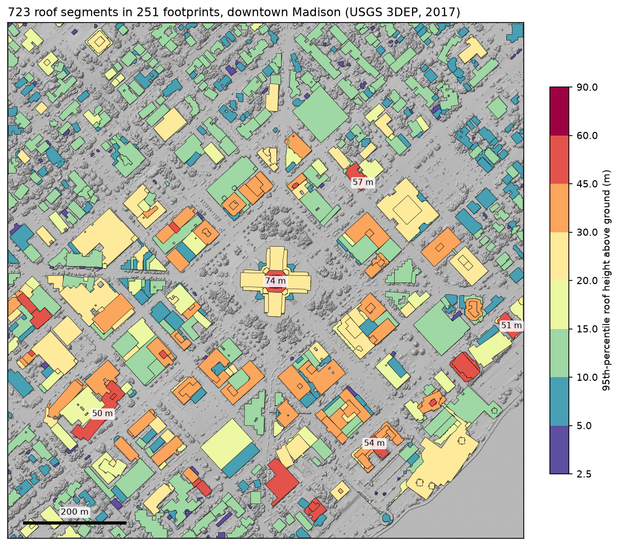
STEP = 3.0 # a jump of more than 3 m within 1 m is a wall between two roofs, not a roof slopeidx = ndimage.distance_transform_edt(~np.isfinite(ndsm_bld), return_distances=False, return_indices=True)roof = ndsm_bld[tuple(idx)]step = ndimage.maximum_filter(roof, size=3) - ndimage.minimum_filter(roof, size=3)core = mask & (step <= STEP)seg, _ = ndimage.label(core)723 roof segments; 117 of 251 footprints were split at height steps > 3.0 mWe keep both layers: footprints (the outline of each connected building mass) and roof segments (parts with one roof level). Which one you want depends on the job. Footprints are better for building coverage, segments for 3D models and solar analysis.
Step 4: polygonise and regularise the outlines
rasterio.features.shapes turns each label into a polygon, but the result follows cell edges. A straight wall at 40° to the grid becomes a 1 m staircase with more than a hundred vertices. Douglas–Peucker simplification alone rounds the corners and leaves walls slightly crooked, so we regularise each building in three ways and keep the best:
- Oriented rectangle. If the polygon fills at least 85% of its minimum rotated rectangle, use the rectangle.
- Orthogonal snapping. Otherwise, find the building’s dominant direction from its minimum rotated rectangle and rotate the building so that direction is horizontal. Re-grid it at 0.5 m in that frame, snap edges within 20° of horizontal or vertical to exact horizontals and verticals, remove jogs shorter than 2.5 m and rotate it back. The result is accepted if its IoU with the original is at least 0.8.
- Simplified. If snapping fails, as it does for curved or many-angled buildings, fall back to a 0.5 m closing plus Douglas–Peucker at 1 m.
def regularise_part(poly): mrr = poly.minimum_rotated_rectangle if poly.area / mrr.area >= RECT_MIN: return mrr, "rectangle" simp = poly.buffer(0.5, join_style="mitre").buffer(-0.5, join_style="mitre").simplify(DP_TOL) theta, origin = dominant_angle(poly), poly.centroid rot = shapely.affinity.rotate(poly.buffer(1, join_style="round").buffer(-1, join_style="round"), -theta, origin=origin) # ... rasterise rot at 0.5 m, polygonise, orthogonal_ring() snaps the edges ... ortho = shapely.affinity.rotate(shapely.make_valid(ortho), theta, origin=origin) if ortho.intersection(poly).area / ortho.union(poly).area >= 0.8: return ortho, "orthogonal" return simp, "simplified"The full orthogonal_ring() function, which merges parallel edges and rebuilds corners as line intersections, is in the script.
footprints: 251 polygons | vertices 136 -> 16 on average | {'orthogonal': 177, 'simplified': 59, 'rectangle': 15} | IoU with staircase median 0.889, min 0.800 | area 371,854 -> 381,536 m²roof segments: 723 polygons | vertices 81 -> 11 on average | {'orthogonal': 484, 'simplified': 216, 'rectangle': 23} | IoU with staircase median 0.884, min 0.615 | area 371,854 -> 377,549 m²Regularisation cuts the vertex count by almost 90% while keeping a median IoU of 0.889 with the staircase. The footprints grow by 2.6% in area, because snapping moves each staircase edge to its average position and the closing fills small notches. For area statistics, the staircase polygons are the more faithful measure of what the lidar saw.
Step 5: building heights from the points
Rasters are convenient for shapes, but heights are better taken from the points themselves. We give every class 6 return a height above the DTM and group by the polygon label of its cell. The median describes a flat roof; the 95th percentile is a robust “top of building” that ignores a few stray points such as antennas, flagpoles and birds; the maximum is the true highest point:
b = cls == 6hb = z[b] - dtm[row[b], col[b]]            # height above ground of every building point

def add_heights(gdf, lab): lab_b = lab[row[b], col[b]] pts = pd.DataFrame({"bid": lab_b, "h": hb})[lab_b > 0] stats = pts.groupby("bid")["h"].agg(n_points="size", h_median="median", h_p95=lambda s: s.quantile(0.95), h_max="max") gdf = gdf.join(stats, on="bid") gdf["area_m2"] = gdf.area gdf["floors_est"] = np.maximum(1, np.round(gdf["h_median"] / 3.5)).astype(int) return gdf251 footprints contain 1,443,984 of 1,474,900 class 6 pointsfootprints: area_m2 h_median h_p95 h_max n_pointsmean 1520.1 10.1 14.4 16.0 5752.950% 402.0 8.6 11.1 12.0 1810.090% 5297.0 18.3 34.0 37.2 16592.0max 20512.0 43.5 57.1 86.3 97667.0
tallest five roof segments by 95th-percentile height: bid area_m2 h_median h_p95 h_max floors_est lon lat 385 584.0 65.4 73.8 86.3 19 -89.38417 43.07469 211 449.0 35.1 56.7 59.8 10 -89.38215 43.07645 621 188.0 52.0 54.1 55.0 15 -89.38171 43.07191 476 1085.0 45.0 50.6 53.1 13 -89.37858 43.07404 536 3385.0 46.6 50.5 52.4 13 -89.38824 43.07231The polygons capture 97.9% of all building points. The median footprint is 402 m² with a 95th-percentile roof at 11.1 m, roughly three storeys. The floors_est column simply divides the median height by 3.5 m. It is a rough guide that works for offices and flats but not for churches, car parks or the Capitol.
Check: the Wisconsin State Capitol
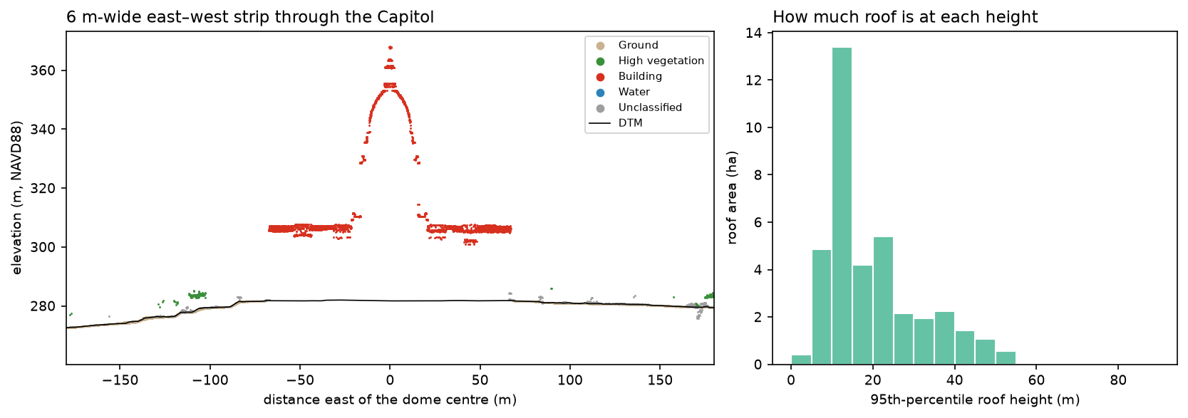
The Capitol is 284 ft 5 in (86.7 m) from the ground floor to the top of the Wisconsin statue on the dome. The script finds the footprint containing the dome centre and the highest building return inside it:
Capitol footprint: 9,486 m², median roof 23.4 m, highest return 86.3 m above ground, 0.8 m from the footprint centroidofficial height 86.7 m: difference -0.4 mthe Capitol footprint was split into 9 roof segmentsThe highest lidar return is 0.4 m below the official height and 0.8 m from the centre of the building. At 5 points/m², a statue a few metres wide gets only a handful of returns, and the very tip is easily missed, so a small underestimate is expected. The profile below shows how clearly the dome stands out:
Step 6: compare with OpenStreetMap buildings
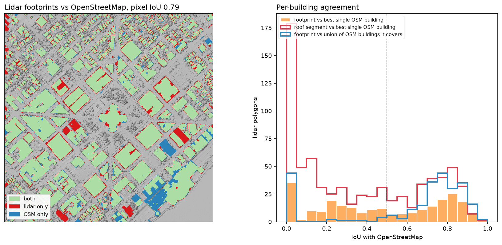
OpenStreetMap is the obvious reference, but it is not ground truth either. It is digitised from aerial imagery of different dates, often by different people. We download all building=* polygons for the same box with osmnx, clip them, and compare in two ways.
Pixel level. We rasterise both layers on the 1 m grid and compute IoU, precision and recall. NAD83 and WGS84 differ by about a metre in the US, so we first test whole-metre shifts of the OSM layer:
osm_r, lid_r = rasterise(osm), rasterise(fp)scores = {(dx, dy): (np.roll(osm_r, (dy, dx), axis=(0, 1)) & lid_r).sum() / (np.roll(osm_r, (dy, dx), axis=(0, 1)) | lid_r).sum() for dx in range(-3, 4) for dy in range(-3, 4)}Object level. For each lidar polygon we find the OSM building with the highest IoU and call it a match if IoU ≥ 0.5. Because one lidar footprint often covers a whole terrace that OSM maps as separate houses, we also compute a many-to-one IoU: each lidar footprint against the union of all the OSM buildings it mostly covers.
601 OSM building polygons in the area, 359,592 m²; 5 have a numeric height tagpixel IoU as downloaded: 0.781; best whole-metre shift +1 m east, -1 m north gives 0.789pixel level: IoU 0.789 | precision 0.857 | recall 0.909
object level (a match is IoU >= 0.5), 601 OSM buildings:                     footprints roof segmentslidar polygons              251           723lidar matched 1:1         46.6%         35.5%OSM matched 1:1           19.5%         42.8%lidar matched many:1      78.9%         46.3%median IoU 1:1            0.465          0.28covering 2+ OSM              99            90
OSM buildings less than 10% covered by lidar footprints: 19, median area 54 m², total 8,741 m²; tags {'yes': 9, 'apartments': 3, 'house': 3}lidar footprints less than 10% covered by OSM: 26, median area 41 m², median p95 height 3.6 m
How to read this:
- The two layers agree on where the buildings are. A pixel IoU of 0.789, with 91% of OSM building area inside a lidar footprint, is a good result for two independent sources.
- They disagree on what a building is. 99 lidar footprints each cover two or more OSM buildings. Scored one-to-one, fewer than half match. Scored against the OSM buildings they cover, 78.9% do.
- Roof segments are closer to OSM’s idea of a building. Splitting at height steps raises the share of OSM buildings with a one-to-one match from 19.5% to 42.8%. It also over-splits some single buildings with stepped roofs, which is why the median IoU per segment falls.
- The leftovers are small. The 19 OSM buildings that the lidar missed have a median area of 54 m², mostly small houses and garages, perhaps hidden by trees or built after 2017. The 26 lidar-only footprints have a median area of 41 m² and a median p95 height of 3.6 m, so they are probably sheds, kiosks and shelters that OSM has not mapped.
Step 7: export a GeoPackage and draw a 3D view
The script writes four layers to one GeoPackage, plus the building nDSM and a CSV of roof-segment heights:
cols = ["bid", "method", "area_m2", "ground_m", "h_median", "h_p95", "h_max", "floors_est", "volume_m3", "n_points", "iou_raw", "iou_osm", "iou_osm_merged", "n_osm"]fp[cols + ["osm_cover", "geometry"]].to_file(gpkg, layer="footprints")sg[cols + ["geometry"]].to_file(gpkg, layer="roof_segments")raw_fp.to_file(gpkg, layer="footprints_staircase")osm.drop(columns=["oid"]).to_file(gpkg, layer="osm_buildings")wrote madison_buildings.gpkg (layers: footprints, roof_segments, footprints_staircase, osm_buildings), ndsm_buildings.tif and roof_segment_heights.csvIn QGIS, open the roof_segments layer and use 2.5D symbology or the 3D map view with h_p95 as the extrusion height. For a quick check in Python, matplotlib’s Poly3DCollection can extrude each roof segment as walls plus a flat roof:
for _, r in sg.iterrows(): geoms = r.geometry.geoms if r.geometry.geom_type == "MultiPolygon" else [r.geometry] h = r["h_p95"] for g in geoms: xy = np.asarray(g.exterior.coords)[:, :2] - [cx, cy] walls = [[(*xy[i], 0), (*xy[i + 1], 0), (*xy[i + 1], h), (*xy[i], h)] for i in range(len(xy) - 1)] roof_poly = [[(px, py, h) for px, py in xy]] ax.add_collection3d(Poly3DCollection(walls + roof_poly, facecolor=SPECTRAL(norm3(h)), edgecolor="#333333", lw=0.1))ax.set_box_aspect((1, 1, 0.22)) # 1000 m x 1000 m x ~100 m: true vertical scale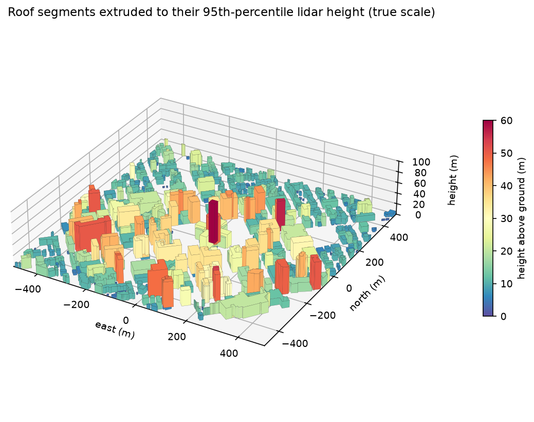
For an interactive version, the same GeoDataFrame works with pydeck’s PolygonLayer and extruded=True, or with deck.gl in the browser.
Pitfalls and limitations
- No class 6, no shortcut. Many lidar datasets, including large parts of USGS 3DEP, classify only ground and leave everything else unclassified. Always count the classes first, as in Step 1. Without a building class you have to separate buildings from trees yourself, for example with PDAL’s
filters.smrfand planarity tests, lidR’ssegment_shapes()or a trained model. - Party walls. Lidar cannot see walls between buildings of the same height, so terraces and city blocks become single footprints. The 3 m step split helps but cannot separate roofs at the same level, and it over-splits stepped roofs. To get one polygon per address you need cadastral or OSM data.
- Edge accuracy. At 5 points/m² a roof edge is only known to about ±0.5 m, and lidar pulses hit overhanging eaves rather than walls. Expect footprints a little larger than the ground-floor walls, and allow for the 2.6% growth from regularisation.
- Point density varies. The horizontal band in Figure 1 has fewer points because of the flight-line overlap. Thin roofs, glass and dark membranes can give sparse or missing returns, which the hole filling partly repairs.
- Date. The lidar is from 2017. Anything built or demolished since then shows up as a disagreement with OSM rather than an error in either source.
- Heights are above the interpolated DTM. On sloping sites, the height of a building depends on where you measure the ground; we use the DTM under each point.
- Overpass can be slow. Public Overpass servers often time out, so the script retries three mirrors with backoff and caches the result.
Frequently asked questions
How do you extract building footprints from LiDAR?
Keep the building-class points (ASPRS class 6) or classify them yourself, grid them to a raster, subtract a ground DTM and keep cells more than about 2–3 m above ground. Clean the mask with morphological closing and opening, label the connected regions and convert them to polygons with rasterio.features.shapes. Then regularise the outlines into straight edges, as in Step 4.
How do you calculate building height from LiDAR?
Subtract the ground elevation (from a DTM built from class 2 points) from the elevation of each roof point, then summarise per footprint. The median is a good roof height for flat roofs, the 95th percentile a robust top-of-building height, and the maximum the highest point, including spires and antennas. Here the maximum on the Wisconsin State Capitol was within 0.4 m of the official 86.7 m.
Can I extract buildings from an unclassified point cloud?
Yes, but you need to classify it first. Ground filters such as SMRF or CSF in PDAL separate ground. Buildings can then be separated from vegetation by planarity, return number (trees produce many multiple returns, roofs few), height and size. Deep-learning models such as PointNet++ or RandLA-Net work well if you have training data. Once you have a building class, the rest of this tutorial applies unchanged.
What point density do I need for building footprints?
Around 2 points/m² is enough to find most buildings larger than a garage, but the edges will be rough. With 5 points/m², as here, footprints of 20 m² and more are reliable and edges are within about half a metre. Denser surveys, such as USGS Quality Level 1 at 8 points/m² or more, give cleaner edges, roof planes and small structures.
How accurate are LiDAR building footprints compared with OpenStreetMap?
In this test the two layers agreed at a pixel IoU of 0.789, with 86% of lidar building area inside OSM buildings and 91% of OSM building area inside lidar footprints. Most differences came from how buildings are split rather than where they are: lidar merges joined buildings and OSM maps them separately. Neither is perfect; lidar has accurate heights and is consistent, while OSM has addresses, uses and detailed outlines drawn from imagery.
Can I do this for a city in the UK?
Yes. The Environment Agency’s National LiDAR Programme publishes point clouds and 1 m DTM and DSM rasters for England under the Open Government Licence. Check which classes the point cloud tiles contain first. If there is no building class, use the DSM minus the DTM as the nDSM and separate buildings from trees with OSM or OS Open Map Local footprints as a mask, or with a planarity test. For Scotland, Wales and Northern Ireland, see the UK data sources.
Next steps
- Start from the basics in LiDAR point clouds in Python with laspy, or turn the nDSM into a printable city model with DEM to STL in Python.
- Use the DTM from Step 2 for hydrology, as in watershed delineation in Python with pysheds, or for slope and aspect with rasterio terrain analysis.
- Join the footprints to OSM attributes with GeoPandas, and speed up overlays across a whole city with fast vector geoprocessing.
- Put the roof segments on an interactive map with Folium, coloured by height.
- Fit planes to the points in each roof segment to get roof pitch and aspect, the starting point for rooftop solar potential.
- Find buildings in aerial imagery alone, with no lidar, in Segment Anything on satellite and aerial imagery.
Data and licences
- Lidar: USGS 3D Elevation Program, WI 4-County Statewide 2017 (tiles A17_0922, A17_0872 and A17_0871). USGS data are in the public domain. Accessed as COPC from the Microsoft Planetary Computer on 14 October 2026.
- Building outlines: © OpenStreetMap contributors, available under the Open Database Licence (ODbL). Accessed via the Overpass API on 14 October 2026.
- Capitol height: 284 ft 5 in (86.7 m), as published by the Wisconsin Department of Administration.
- Code:
building_footprints.py, tested with Python 3.12.0, laspy 2.7.0, lazrs 0.8.2, numpy 2.5.4, scipy 1.18.1, rasterio 1.5.2, shapely 2.2.0, geopandas 1.2.0 and osmnx 2.1.1.
Key terms
- ASPRS class 6
- The LAS classification code for building points. Others include 2 (ground), 5 (high vegetation) and 9 (water). Whether a dataset has class 6 depends on the vendor and the project specification.
- nDSM
- Normalised digital surface model: the surface height minus the bare-earth DTM, so each cell holds a height above ground rather than above sea level.
- Regularisation
- Turning a jagged, pixel-based outline into a clean building polygon with straight, mostly perpendicular edges, as a human digitiser would draw it.
- IoU
- Intersection over union: the shared area of two shapes divided by their combined area. 1 means identical, 0 means no overlap. 0.5 is a common threshold for calling two objects a match.
- COPC
- Cloud Optimised Point Cloud: a LAZ file organised as an octree, so a client can read just the points inside a box over HTTP without downloading the whole tile.
- Roof segment
- Part of a footprint whose roof is continuous in height. Here a jump of more than 3 m between neighbouring cells starts a new segment.
Data for this tutorial
- USGS 3D Elevation Program (3DEP) · Classified lidar point clouds, WI 4-County Statewide 2017
- Microsoft Planetary Computer · The 3dep-lidar-copc collection, streamed as COPC
- OpenStreetMap · Building outlines for the comparison
- Overture Maps · An alternative open building layer
Licences and formats for each source are listed in the GIS data sources catalogue.