Watershed delineation in Python with pysheds: the River Derwent above Ladybower

Short answer: to delineate a watershed in Python, load a DEM with pysheds, then fill pits and depressions and resolve flats so every cell can drain. Compute D8 flow direction and flow accumulation, and snap your outlet to the nearest cell with large accumulation. Then call grid.catchment() for that point and convert the mask to a polygon with rasterio.features.shapes. For the stream network, keep cells whose upstream area exceeds a threshold (here 0.5 km²) and run grid.stream_order() for Strahler order. Always check the result against an official boundary or a published catchment area if one exists.

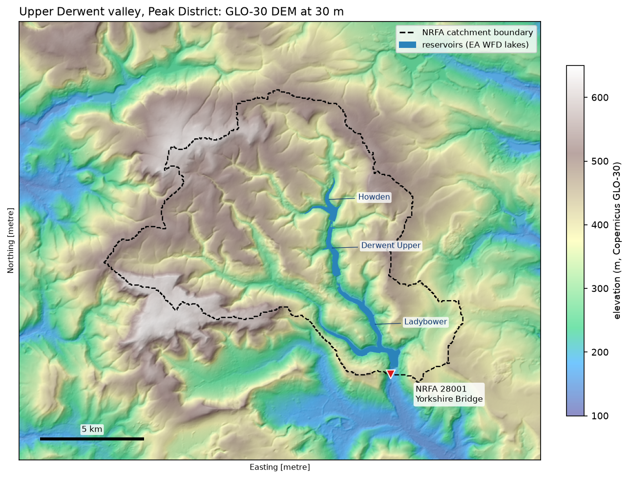
We delineate a real, well-documented catchment: the River Derwent above Yorkshire Bridge in the Peak District, just below Ladybower dam. This is the catchment of Howden, Derwent and Ladybower reservoirs, the same reservoirs we monitored from space in the Sentinel-2 reservoir water quality tutorial. The UK National River Flow Archive (NRFA) gauges the river there as station 28001 and publishes its catchment boundary, so we can measure how close a free 30 m DEM gets.

You will learn how to:

1. get a gauge location and the official catchment from the NRFA web services;
2. download the Copernicus GLO-30 DEM and reproject it to British National Grid;
3. condition the DEM: fill pits and depressions, and resolve flats;
4. compute D8 flow direction and flow accumulation;
5. snap the pour point and delineate the catchment polygon and its area;
6. extract a stream network with Strahler order and drainage density, and test the threshold;
7. compare the result with the NRFA boundary and the Environment Agency’s Water Framework Directive catchments, and export a GeoPackage.

All outputs below are real results from watershed_delineation.py, run on 14 October 2026 with Python 3.12, pysheds 0.5, numpy 2.5.4, rasterio 1.5.2 and geopandas 1.2.0.

Step 1: the gauge and the official answer

Start with the answer you want to reproduce. The NRFA station-information API returns the gauge’s grid reference and catchment descriptors as JSON, and its GeoServer serves the official catchment boundary over WFS:

STATION = 28001                       # River Derwent at Yorkshire Bridge, below Ladybower dam
r = requests.get("https://nrfaapps.ceh.ac.uk/nrfa/ws/station-info",
                 params={"station": STATION, "format": "json-object", "fields": "all"}, timeout=60)
info = r.json()["data"][0]
gx, gy = info["easting"], info["northing"]

r = requests.get("https://hydrologygeoserver.ceh.ac.uk/geoserver/ows",
                 params={"service": "WFS", "version": "2.0.0", "request": "GetFeature",
                         "typename": "NRFA:NRFA_catchments", "CQL_FILTER": f"ID={STATION}",
                         "outputformat": "application/json", "srsname": "EPSG:27700"}, timeout=60)
nrfa = gpd.read_file(io.StringIO(r.text))     # the script caches both responses in data/

=== NRFA station 28001: Derwent at Yorkshire Bridge ===
gauge at British National Grid 419810 E, 385090 N | catchment area 126.0 km² (IHDTM 126.71 km²) | altitude 160.0–631.2 m | drainage density 1.138 km/km²
NRFA boundary polygon: 126.70 km²

The NRFA publishes two areas: 126.0 km² is the official catchment area, and 126.71 km² is the area derived from the 50 m Integrated Hydrological DTM (IHDTM), which is also the area of the boundary polygon.

Step 2: download and reproject the DEM

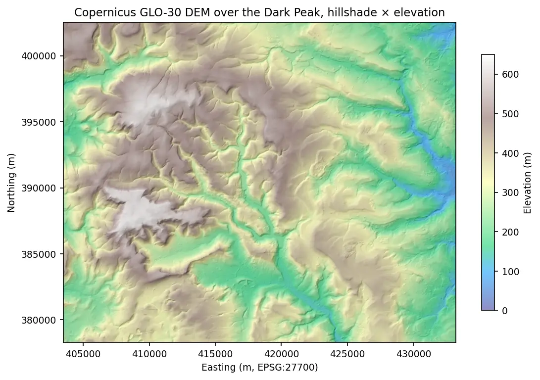
We use Copernicus GLO-30, a free global DEM with 1 arc-second (about 30 m) cells, from the Planetary Computer. Hydrology needs square cells in metres, so we reproject it to British National Grid (EPSG:27700) at 30 m for a 25 km × 21 km box around the catchment:

RES = 30.0
X0, Y0, X1, Y1 = 402_000, 381_000, 427_000, 402_000   # 25 km x 21 km of the Dark Peak in BNG
lon0, lat0, lon1, lat1 = Transformer.from_crs(27700, 4326, always_xy=True).transform_bounds(X0, Y0, X1, Y1)
cat = pystac_client.Client.open("https://planetarycomputer.microsoft.com/api/stac/v1",
                                modifier=planetary_computer.sign_inplace)
items = list(cat.search(collections=["cop-dem-glo-30"], bbox=[lon0, lat0, lon1, lat1]).items())
for item in items:
    with rasterio.open(item.assets["data"].href) as src:
        reproject(rasterio.band(src, 1), part, dst_transform=from_origin(X0, Y1, RES, RES),
                  dst_crs="EPSG:27700", dst_nodata=np.nan, resampling=Resampling.bilinear)

grid = Grid.from_raster(str(dem_path))
dem = grid.read_raster(str(dem_path))

=== DEM ===
833 x 700 cells of 30 m (EPSG:27700) | elevation 129.7–634.5 m | missing cells 0

Make the box comfortably larger than the catchment. If the divide touches the edge of the DEM, part of the catchment is cut off and nothing warns you.

Step 3: condition the DEM

Real DEMs contain closed hollows: single-cell pits from noise, and larger depressions from errors, bridges, dams and genuine features such as quarries. Water flowing into a hollow has nowhere to go, so the flow network breaks. pysheds fixes this in three steps:

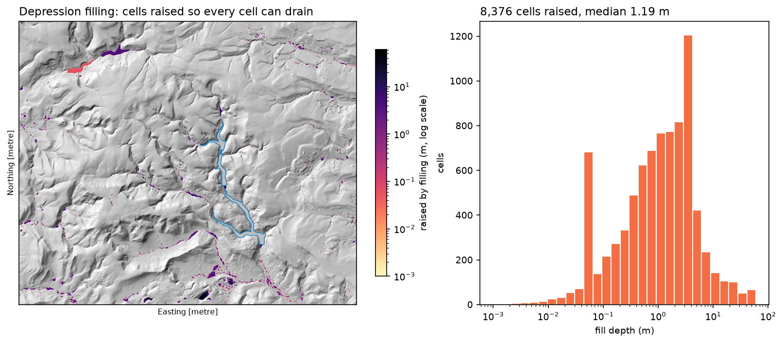
pit_filled = grid.fill_pits(dem)
pits = np.asarray(pit_filled) > np.asarray(dem)          # copy now: the next step can modify in place
flooded = grid.fill_depressions(pit_filled)
inflated = grid.resolve_flats(flooded)
fill = np.asarray(flooded) - np.asarray(dem)

single-cell pits raised: 1,440
cells raised by depression filling (beyond the pits): 6,936 (1.2%) | max fill 60.2 m | volume 22.10 million m³
deepest fill at (415635, 381525), DEM 224.0 m raised to 284.2 m
flat cells after filling: 14,869; resolve_flats adds a tiny gradient so they drain

Filling raised 8,376 cells. Most changes are under a few metres, but the deepest is 60 m at the bottom edge of the box, near the Hope cement works quarry, outside our catchment. Filling turns every depression into a flat lake surface, so resolve_flats then adds a tiny gradient across the 14,869 flat cells so that water drains towards the outlet instead of stopping.

Step 4: flow direction and flow accumulation

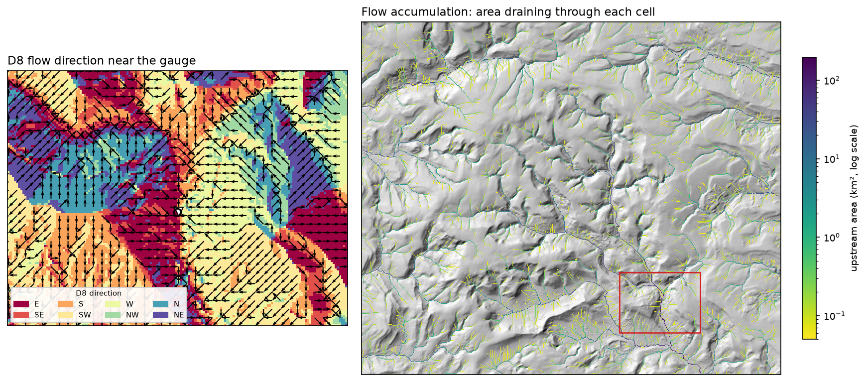
D8 sends all the water in each cell to its steepest downhill neighbour. pysheds encodes the eight directions as powers of two, and the dirmap argument says which code means which direction (here the ESRI convention). Flow accumulation counts how many cells drain through each cell; multiplied by the cell area, it gives the upstream area:

DIRMAP = (64, 128, 1, 2, 4, 8, 16, 32)           # N, NE, E, SE, S, SW, W, NW (ESRI convention)
fdir = grid.flowdir(inflated, dirmap=DIRMAP)
acc = grid.accumulation(fdir, dirmap=DIRMAP)
acc_km2 = np.asarray(acc) * RES ** 2 / 1e6

largest upstream area in the grid: 196.3 km²
flow directions: E 11.9%, SE 12.3%, S 15.0%, SW 12.0%, W 11.1%, NW 9.6%, N 14.6%, NE 13.5%

The largest value, 196.3 km², is where the Derwent leaves the bottom of our box after the River Noe joins it. If you use a different dirmap in different calls, the results are garbage without any error, so define it once and pass it everywhere.

Step 5: snap the pour point

A gauge’s published coordinates rarely fall exactly on the DEM’s river cell. One cell to the side, and you get the catchment of a hillside a few hundred metres square. The standard fix is to snap the point to the nearest cell whose upstream area is above a threshold suited to the river:

SNAP_KM2 = 50                                       # snap to a cell that drains at least 50 km²
sx, sy = grid.snap_to_mask(acc > SNAP_KM2 * 1e6 / RES ** 2, (gx, gy))

gauge cell drains 126.37 km² before snapping
snapped to (419790, 385080), 22 m from the gauge; that cell drains 126.4 km²

Here the gauge already sits on the right cell and snapping moves it only 22 m. That is not always the case. Use a threshold well below the expected catchment area but well above the tributaries next to the outlet. If it is too low, the point can snap to a side stream.

Step 6: delineate the catchment

With a conditioned flow-direction grid and a good pour point, the catchment is one call. We turn the mask into a polygon and compare it with the NRFA boundary:

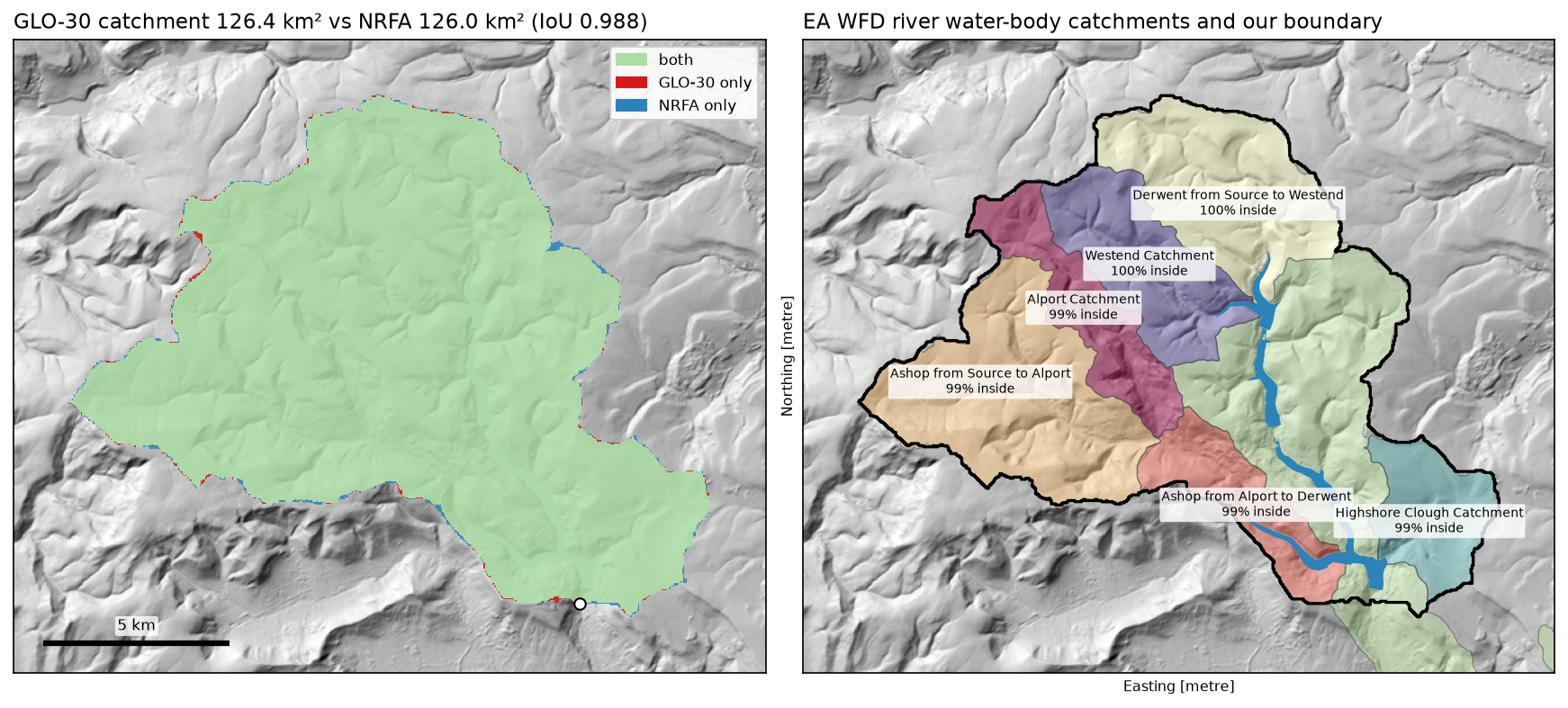
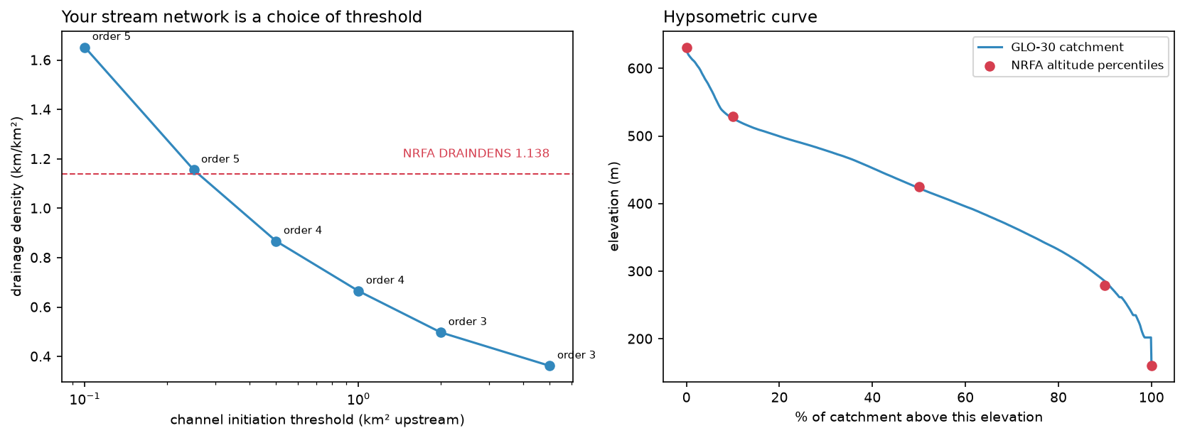
catch = grid.catchment(x=sx, y=sy, fdir=fdir, dirmap=DIRMAP, xytype="coordinate")
cmask = np.asarray(catch).astype(bool)
area = cmask.sum() * RES ** 2 / 1e6
polys = [shape(g) for g, v in features.shapes(cmask.astype("uint8"), mask=cmask,
                                                transform=grid.affine, connectivity=8)]
ours = gpd.GeoDataFrame({"area_km2": [round(area, 2)]}, geometry=[shapely.union_all(polys)], crs=27700)
ref = nrfa.geometry.iloc[0]
inter, union = ours.geometry.iloc[0].intersection(ref).area, ours.geometry.iloc[0].union(ref).area

delineated area 126.38 km² vs NRFA 126.0 km² (+0.3%); vs NRFA boundary polygon 126.70 km²
IoU with the NRFA boundary 0.988 | only in ours 0.61 km² | only in NRFA 0.94 km²
              min    10%  median    90%    max
GLO-30 (m)  162.9  285.0   422.8  525.8  629.1
NRFA (m)    160.0  279.3   424.7  528.7  631.2
mean elevation 417 m (NRFA ALTBAR 416 m)
longest flow path 19.9 km; mean flow path 11.34 km (NRFA DPLBAR 11.21 km)

That is a very good match. The area is within 0.3% of the official figure and the IoU with the official boundary is 0.988. The elevation percentiles are within 6 m and the mean flow-path length (DPLBAR) within 1.2%. The disagreements are slivers along the divide, where the moorland tops are so flat that 30 m and 50 m DEMs put the watershed in slightly different places.

A second check: Environment Agency WFD catchments

The Environment Agency divides England’s rivers into Water Framework Directive (WFD) water bodies, each with its own catchment, on the Catchment Data Explorer. Six of them lie upstream of Ladybower dam:

            id                                         name  kind  area_km2  share_inside
GB104028057960               Derwent from Source to Westend river     20.56         0.995
GB104028057950          Westend Catchment (trib of Derwent) river     14.92         0.999
GB104028057930                  Ashop from Source to Alport river     27.82         0.990
GB104028057940             Alport Catchment (trib of Ashop) river     11.34         0.992
GB104028057910                 Ashop from Alport to Derwent river     10.19         0.992
GB104028057900 Highshore Clough Catchment (trib of Derwent) river      9.84         0.994
GB104028057880                  Derwent from Westend to Wye river    142.84         0.219
    GB30432299                             Howden Reservoir  lake      0.62         1.000
    GB30432359                      Derwent Upper Reservoir  lake      0.70         1.000
    GB30432459                          Ladybower Reservoir  lake      1.97         1.000
river water bodies more than half inside: 6, 94.67 km² together; IoU with our catchment 0.740

Every upstream water body is 99–100% inside our boundary. They add up to only 94.67 km², though, because the main-stem Derwent water body runs from Westend all the way down to the River Wye (142.84 km²). Only 22% of it is above the gauge, and it fills the green gap down the middle of the right-hand map. WFD water bodies are management units, not gauge catchments, so they make a good consistency check but not a replacement for the NRFA boundary.

Step 7: stream network and Strahler order

A stream network from a DEM is simply the cells whose upstream area exceeds a channel initiation threshold. pysheds then traces the branches as lines and computes Strahler order:

STREAM_KM2 = 0.5                                    # a channel starts where 0.5 km² drains to a cell
BOOL_VF = ViewFinder(affine=grid.affine, shape=grid.shape, crs=grid.crs, nodata=False)   # for mask rasters
streams = Raster((acc_km2 > STREAM_KM2) & cmask, viewfinder=BOOL_VF)
# pysheds also labels the cell just past the outlet (order + 1), so keep only stream cells
order = np.where(np.asarray(streams), np.asarray(grid.stream_order(fdir, streams, dirmap=DIRMAP)), 0)
branches = grid.extract_river_network(fdir, streams, dirmap=DIRMAP)

Each branch takes the most common order of its cells, and the script builds a GeoDataFrame of lines with lengths:

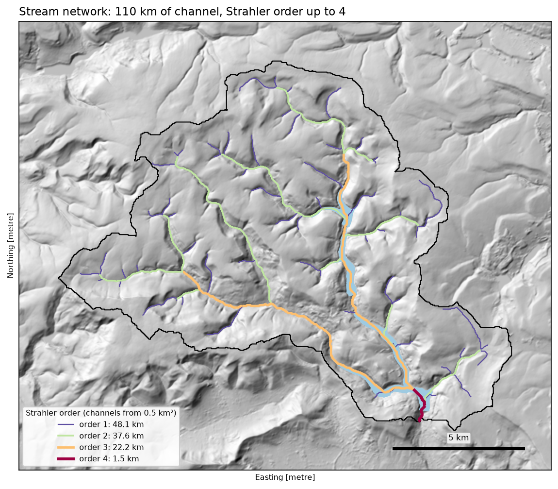
channel heads at 0.5 km²: 127 segments, 109.5 km, highest Strahler order 4
          segments  length_km
strahler
1               64       48.1
2               44       37.6
3               17       22.2
4                2        1.5
drainage density 0.867 km/km² (NRFA DRAINDENS 1.138)

The upper Derwent and the Ashop are both order 3. They join in Ladybower, only 1.5 km above the dam, which is why order 4 is so short.

How much does the threshold matter?

A lot. The NRFA’s drainage density of 1.138 km/km² comes from a 1:50,000 river map, not from a DEM, and nothing in the DEM tells you where a real channel starts. Re-running with different thresholds shows the effect:

 threshold_km2  drainage_density  max_strahler
          0.10             1.652             5
          0.25             1.155             5
          0.50             0.867             4
          1.00             0.665             4
          2.00             0.497             3
          5.00             0.362             3

A threshold of about 0.25 km² reproduces the NRFA drainage density in this valley. The highest Strahler order changes from 3 to 5 across the range, so always report the threshold with any stream order or drainage density. A better approach for a real study is to calibrate the threshold against mapped channel heads or a river layer such as OS Open Rivers.

Step 8: export

The script writes the catchment, streams, both reference layers and the pour points to one GeoPackage, plus the flow-accumulation raster in km²:

ours.to_file(gpkg, layer="catchment")
net.to_file(gpkg, layer="streams")
nrfa.drop(columns=["id"], errors="ignore").to_file(gpkg, layer="nrfa_catchment")
wfd.to_file(gpkg, layer="ea_wfd_waterbodies")

wrote derwent_catchment.gpkg (layers: catchment, streams, nrfa_catchment, ea_wfd_waterbodies, pour_point) and flow_accumulation_km2.tif

The NRFA layer has both ID and id columns, and GeoPackage field names are case-insensitive, so writing it unchanged raises FieldError: Error adding field 'ID'. Dropping one of them fixes it.

Pitfalls and limitations

• GLO-30 is a surface model. Copernicus GLO-30 is a DSM: it includes trees and buildings. In the open moorland of the Dark Peak that hardly matters, but in wooded or urban catchments, blocks of forest and buildings act as dams. Use a bare-earth DTM where you can. For England, the Environment Agency’s 1 m lidar composite DTM is free from the Defra Survey Data Download. Resample it to 5–10 m first, or the flow grid becomes huge and dominated by walls and ditches.
• Filling is not always right. Depression filling assumes every hollow is an error. Real sinks, such as quarries, karst and lakes with no outlet, get filled too, and in flat areas filled DEMs can send water along the wrong route. Breaching (carving through the obstruction), as in WhiteboxTools’ BreachDepressionsLeastCost, often gives more realistic paths, especially where roads and embankments cross valleys.
• Reservoirs and dams. A dam is a wall across the valley in the DEM, and the reservoir surface is a big flat. Here the gauge is below the dam so it works, but if you put a pour point in the middle of a reservoir, check that the flats were resolved towards the real outlet.
• Natural versus real catchment. The NRFA notes that the Derwent has diversions within the basin (Ashop), imports (water piped in from the River Noe, outside the catchment) and public water supply exports. A DEM gives the topographic catchment only. The water arriving at the gauge comes from a slightly different area, and the flow is dominated by Ladybower releases.
• D8 limitations. D8 cannot split flow, so on smooth slopes it draws parallel straight lines and it overestimates convergence on ridges. That does not affect catchment boundaries much, but for wetness indices or erosion modelling, use D-infinity or MFD (grid.flowdir(..., routing="dinf") in pysheds).
• Resolution at the divide. On flat moorland plateaus the exact watershed is uncertain by tens to hundreds of metres. The 0.61 km² and 0.94 km² slivers in Step 6 are that uncertainty, not errors in either source.
• pysheds and NumPy. pysheds 0.5 needs the np.in1d = np.isin shim with NumPy 2.4 or later, and it uses numba, so the first run compiles functions and takes longer.

Frequently asked questions

How do you delineate a watershed in Python?

Load a DEM with pysheds.grid.Grid.from_raster, fill pits and depressions and resolve flats, then compute D8 flow direction and flow accumulation. Snap your outlet to a high-accumulation cell with grid.snap_to_mask, and call grid.catchment(x, y, fdir) to get a boolean catchment mask. Convert the mask to a polygon with rasterio.features.shapes and save it with GeoPandas. Steps 3 to 6 above show the full code.

What DEM is best for watershed delineation?

Use the best bare-earth DTM you can get at a sensible resolution for the catchment size. For catchments of tens to hundreds of square kilometres, a 10–30 m DEM is enough: Copernicus GLO-30, as here, is free worldwide and matched the official boundary at an IoU of 0.988. For small catchments, urban drainage or flat land, use lidar DTMs such as the Environment Agency’s 1 m composite in England or USGS 3DEP in the US, resampled to a few metres.

What is the difference between pysheds and WhiteboxTools?

pysheds is a pure-Python library (NumPy and numba) with a compact API for flow direction, accumulation, catchments and stream networks, which makes it easy to use in a notebook. WhiteboxTools (and its whitebox-workflows Python package) is a large compiled toolbox with hundreds of terrain tools, including depression breaching, more flow algorithms, and tools for watershed sets, basins and stream ordering. It is faster on large rasters. Both give very similar catchment boundaries for a well-conditioned DEM.

Why is my delineated watershed tiny?

Almost always because the pour point is not on the river cell in the DEM. A point one cell to the side of the channel drains only its own hillside. Snap the point to the flow-accumulation network first, as in Step 5, with a threshold appropriate for the river size. Also check that you use the same dirmap for flowdir, accumulation and catchment.

How do I choose the flow accumulation threshold for streams?

There is no universal value. Common starting points are 0.1–1 km² of upstream area for a 30 m DEM. Calibrate it by comparing drainage density with a mapped river network (here, 0.25 km² reproduces the NRFA value), or by checking channel heads on aerial imagery. Report the threshold, because stream order and drainage density depend directly on it.

Where can I get official catchment boundaries in the UK?

The National River Flow Archive publishes catchment boundaries for its gauging stations through a WFS and on each station page. The Environment Agency’s Catchment Data Explorer publishes WFD river and lake water-body catchments for England under the Open Government Licence. For Scotland, SEPA publishes river basin and water-body catchments. For the rest of the world, HydroSHEDS and its HydroBASINS layer give consistent nested basins from a 90 m DEM.

Next steps

• Look inside the reservoirs this catchment feeds in monitoring reservoir water quality with Sentinel-2, and relate colour to the peat cover upstream.
• Add slope, aspect and hillshade maps of the catchment with DEM terrain analysis in rasterio, or print it in 3D with DEM to STL in Python.
• Swap GLO-30 for a lidar DTM. Our building footprints from LiDAR tutorial shows how to build one from a classified point cloud.
• Delineate every NRFA gauge in a region in a loop, and compare all the areas with the published ones using GeoPandas.
• Put the catchment and stream network on an interactive web map with Folium.

Data and licences

• DEM: Copernicus DEM GLO-30, © DLR e.V. 2010–2014 and © Airbus Defence and Space GmbH 2014–2018, provided under COPERNICUS by the European Union and ESA; all rights reserved, free to use under the Copernicus DEM licence. Accessed from the Microsoft Planetary Computer on 14 October 2026.
• Gauging station data and catchment boundary: National River Flow Archive, UK Centre for Ecology & Hydrology, station 28001 Derwent at Yorkshire Bridge. NRFA data are available under the NRFA terms and conditions. Accessed on 14 October 2026.
• WFD water bodies: Environment Agency Catchment Data Explorer, © Environment Agency, licensed under the Open Government Licence v3.0. Accessed on 14 October 2026.
• Code: watershed_delineation.py, tested with Python 3.12.0, pysheds 0.5, numba 0.68.0, numpy 2.5.4, rasterio 1.5.2, geopandas 1.2.0, shapely 2.2.0 and pyproj 3.8.0.