Viewshed analysis in Python: line of sight and a wind farm ZTV with GDAL and numpy
Run a viewshed analysis in Python on a real DEM: compute what one wind turbine can see with gdal.ViewshedGenerate, rebuild the same line-of-sight algorithm in numpy, correct for earth curvature and refraction, build a cumulative zone of theoretical visibility (ZTV) from 26 turbines, draw line-of-sight profiles, and measure how much trees and buildings in a LiDAR DSM shrink a bare-earth viewshed.
- Level
- Intermediate
- Tested with
- Python 3.12
- Source code
- Download scripts
Key takeaways
- gdal.ViewshedGenerate computes a 30 km viewshed on a 2,068 × 2,068 cell DEM in 0.05 s. A 30-line numpy ray caster gives the same answer for 98.5% of cells (kappa 0.962), so you can trust and adapt either.
- Earth curvature matters beyond about 10 km: the ground drops 7.8 m at 10 km and 70.6 m at 30 km. Ignoring it overstates one turbine's visible area by 6% (802 against 758 km²).
- A cumulative viewshed of all 26 Scout Moor turbines shows at least one blade tip from 36.0% of the 30 km circle. Bury sees 25 tips, while Rawtenstall, 5.3 km away in the next valley, sees none.
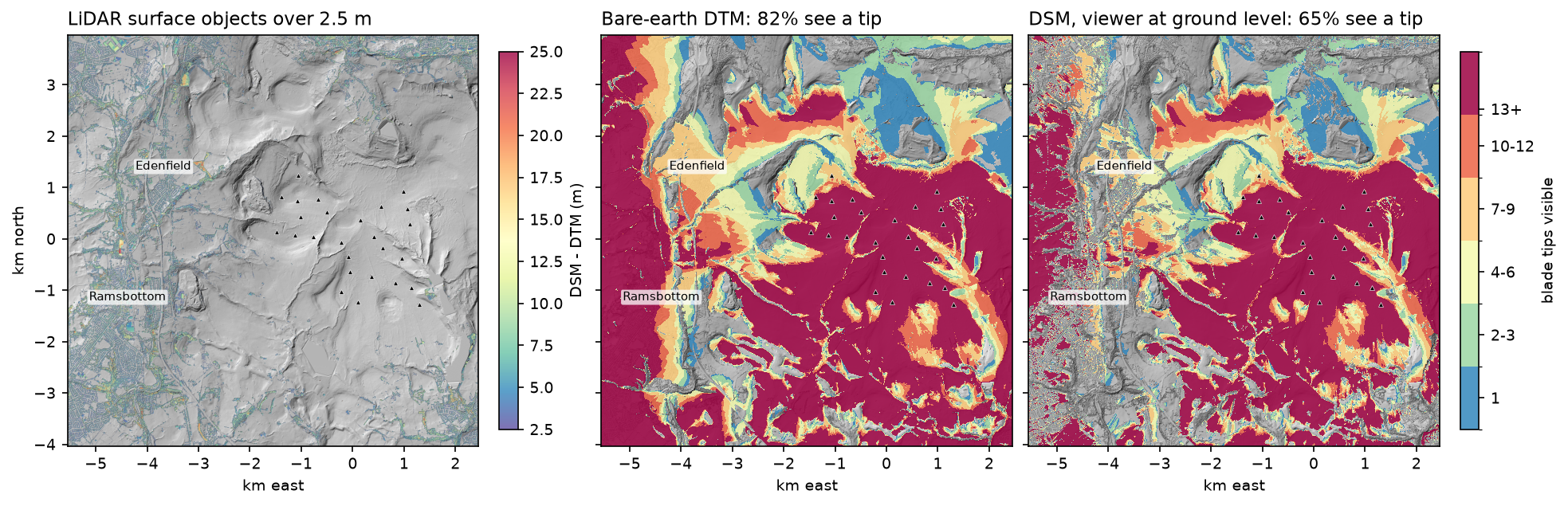
- Surface model choice changes the answer: on Environment Agency LiDAR, 81.7% of the 8 km × 8 km window sees a tip over bare earth (DTM), but only 64.7% once trees and buildings (DSM) are in the way.
Before you start
- Basic numpy and raster concepts: a DEM as a 2D array with a geotransform. Terrain analysis with rasterio is a good warm-up
- Python 3.10+ with GDAL 3.10 or later (Python bindings), numpy, requests, pystac-client, planetary-computer and matplotlib
- An internet connection: the DEM comes from the Microsoft Planetary Computer, the LiDAR from the Environment Agency and the turbine positions from OpenStreetMap, all without an account
Short answer: to run a viewshed analysis in Python, open a DEM with GDAL and call gdal.ViewshedGenerate(band, "MEM", "", [], x, y, observer_height, target_height, 1, 0, 0, -1, 0.85714, gdal.GVM_Edge, max_distance). It returns a raster where 1 means visible and 0 means hidden. The 0.85714 coefficient corrects for earth curvature and atmospheric refraction, which you need beyond a few kilometres. For a cumulative viewshed (for example how many wind turbines are visible from each place), run one viewshed per observer and add the rasters. A line-of-sight check between two points is the same test along a single profile: sample the DEM, lower it for curvature, and see whether the straight sightline ever dips below the ground. Whether you use a bare-earth DTM or a surface DSM with trees and buildings can change the answer by a third.
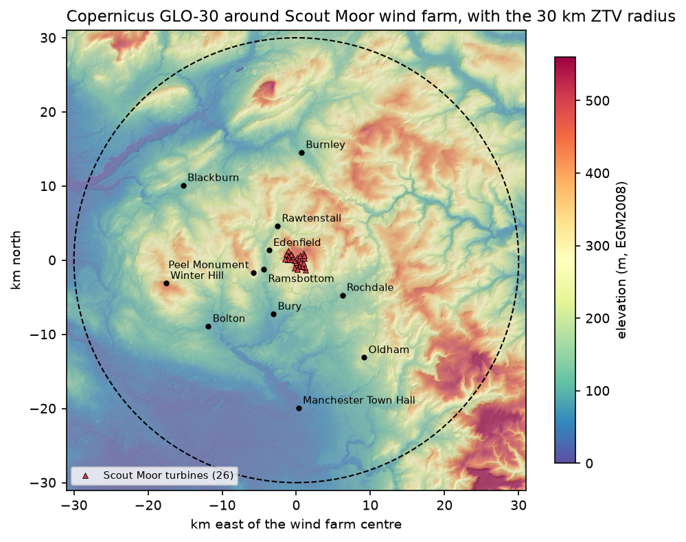
In this tutorial we build a zone of theoretical visibility (ZTV) for Scout Moor wind farm, 26 turbines on the moors between Rochdale, Bury and Rossendale in Greater Manchester and Lancashire. We use the free Copernicus GLO-30 DEM for the 30 km study area and Environment Agency LiDAR for a detailed DTM and DSM comparison.
You will learn how to:
- get turbine positions from OpenStreetMap and a 30 m Copernicus DEM on the British National Grid;
- compute a viewshed with
gdal.ViewshedGenerateand handle its cropped output; - write the same line-of-sight algorithm in numpy and check it against GDAL;
- measure the effect of earth curvature and refraction;
- build a cumulative viewshed (ZTV) from 26 turbines, for blade tips and hubs;
- draw line-of-sight profiles to explain why a place can or cannot see a turbine;
- compare a bare-earth DTM with a DSM from LiDAR, and see how trees and buildings block views.
All outputs below are real results from viewshed_analysis.py, run on 23 October 2026 with Python 3.12.0, GDAL 3.13.3, numpy 2.5.4 and matplotlib 3.11.2.
What is a viewshed?
A viewshed answers “what can be seen from here?” For every cell in a DEM, the algorithm draws a straight line from the observer’s eye to the target, a point at some height above that cell, and checks whether the terrain gets in the way. Typical uses are:
- Wind farm and mast ZTVs for landscape and visual impact assessment;
- telecoms and radio coverage (with extra rules for Fresnel zones);
- viewpoint and summit panoramas, and the planning of new paths and lookouts;
- military and security questions such as “where can this camera see?”;
- archaeology, where intervisibility between hillforts or cairns is a classic study.
Visibility is close to reciprocal: if a 2 m viewer can see a 100 m turbine tip, an observer at the tip can see the 2 m point. So we run the viewshed from each turbine tip to a 2 m eye height, which is the usual way to build a ZTV and needs one run per turbine rather than one per cell.
Step 1: turbine positions from OpenStreetMap
Scout Moor has 26 Nordex N80 2.5 MW turbines with a 60 m hub and 40 m blades, so 100 m to the blade tip. OpenStreetMap maps each one as a power=generator node, so a single Overpass query gets them:
TIP_H, HUB_H = 100.0, 60.0       # Nordex N80 at Scout Moor: 60 m hub + 40 m blade = 100 m to blade tipEYE_H = 2.0                      # viewer eye height used in UK landscape guidance (about 1.5-2 m)RADIUS = 30_000                  # ZTV radius for turbines of 86-100 m to blade tip (NatureScot guidance)
QUERY = """[out:json][timeout:60];node["power"="generator"]["generator:source"="wind"]["generator:output:electricity"="2.5 MW"] (53.62,-2.32,53.68,-2.18);out;"""turbines = overpass(QUERY, DATA / "scout_moor_turbines.json") # tries three Overpass mirrors, then cachestx, ty = np.array([to_bng(e["lat"], e["lon"]) for e in turbines]).Tturbines: 26 | E 382070..384848 | N 416758..419274wind farm centre E 383550 N 418030 | nearest-neighbour spacing 281..495 mThe 30 km radius follows the NatureScot guidance on visual representation of wind farms, which scales the ZTV radius with turbine height (30 km for turbines of 86–100 m to tip). It is widely used in England too.
Step 2: a 30 m Copernicus DEM on the British National Grid
Viewsheds need square cells in metres, so we warp the Copernicus GLO-30 tiles from the Planetary Computer straight into British National Grid (EPSG:27700) at 30 m, with a 1 km margin around the 30 km circle. gdal.Warp reads the cloud-optimised GeoTIFFs over HTTP and mosaics them in one call:
catalog = pystac_client.Client.open("https://planetarycomputer.microsoft.com/api/stac/v1", modifier=planetary_computer.sign_inplace)items = list(catalog.search(collections=["cop-dem-glo-30"], bbox=[-2.79, 53.33, -1.69, 53.98]).items())gdal.Warp(str(dem_path), ["/vsicurl/" + it.assets["data"].href for it in items], dstSRS="EPSG:27700", outputBounds=BOUNDS, xRes=CELL, yRes=CELL, resampleAlg="bilinear", outputType=gdal.GDT_Float32, creationOptions=["COMPRESS=DEFLATE", "TILED=YES"])grid 2068 x 2068 cells of 30 m | elevation 1.0..634.5 mturbine base elevation (GLO-30): 352..472 m, tips at 452..572 m30 km study circle: 2,828 km2The turbines stand at 352–472 m on a moorland plateau. To the south, the land falls to the Manchester plain at under 100 m; to the north lie the Rossendale valleys and the Forest of Bowland beyond.
Step 3: one viewshed with gdal.ViewshedGenerate
GDAL has had a viewshed tool (gdal_viewshed on the command line) since version 3.1. The Python function takes the band, the observer coordinates in the raster’s CRS, the observer and target heights, the output values for visible, invisible, out-of-range and nodata cells, the curvature coefficient, a mode and a maximum distance:
def gdal_viewshed(band, x, y, obs_h, tgt_h, curv=CURV, max_dist=RADIUS, height_mode=gdal.GVOT_NORMAL,                  shape=dem.shape, gt=GT):    """Run GDAL's viewshed in memory and paste the result (cropped to max_dist) onto the full grid."""    oor = 0 if height_mode == gdal.GVOT_NORMAL else 1e9     # out of range: never visible    out = gdal.ViewshedGenerate(band, "MEM", "", [], x, y, obs_h, tgt_h, 1, 0, oor, -1, curv,                                gdal.GVM_Edge, max_dist, heightMode=height_mode)    a = out.GetRasterBand(1).ReadAsArray()    ogt = out.GetGeoTransform()    r0, c0 = int(round((gt[3] - ogt[3]) / -gt[5])), int(round((ogt[0] - gt[0]) / gt[1]))    fill = 1e9 if height_mode != gdal.GVOT_NORMAL else 0    full = np.full(shape, fill, dtype="float32")    full[r0:r0 + a.shape[0], c0:c0 + a.shape[1]] = a    return full
vs_gdal = gdal_viewshed(band, tx[T], ty[T], TIP_H, EYE_H) == 1
Two details trip people up. First, when you set maxDistance, GDAL crops the output to the bounding box of that distance, so its geotransform differs from the input’s. We paste it back onto the full grid so that viewsheds from different turbines line up. Second, the band’s parent dataset must stay referenced while GDAL uses the band, or Python may free it and crash.
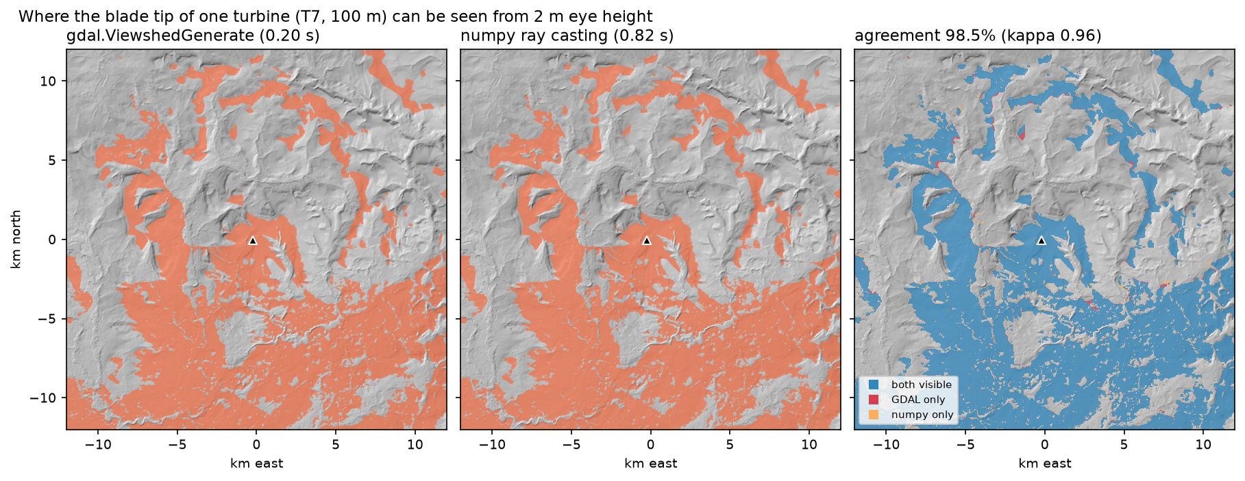
turbine T7 at E 383329 N 417967, base 401 m, observer = blade tip 100 mGDAL viewshed: 0.05 s | tip visible from 758 km2 = 26.8% of the 30 km circleStep 4: the same viewshed in numpy
To understand what GDAL does, or to change the rules (a different visibility test, a vegetation penalty, or GPU arrays), it helps to write the algorithm yourself. The idea is ray casting. Cast a ray from the observer to every edge cell of the square around it. Walk along each ray, keeping the steepest slope from the eye to the ground seen so far. A cell is visible if the slope from the eye to the target above it is at least that running maximum. np.maximum.accumulate does the walk for all rays at once:
def numpy_viewshed(z, r0, c0, obs_h, tgt_h, cell, curv=CURV, max_dist=RADIUS): n = int(max_dist / cell) + 1 edge = np.arange(-n, n + 1) ends = np.concatenate([np.c_[np.full_like(edge, -n), edge], np.c_[np.full_like(edge, n), edge], np.c_[edge, np.full_like(edge, -n)], np.c_[edge, np.full_like(edge, n)]]) k = np.arange(1, n + 1) / n # n steps: at most one cell per step in each axis rr = np.rint(r0 + ends[:, :1] * k).astype(int) # rays x steps cc = np.rint(c0 + ends[:, 1:] * k).astype(int) ok = (rr >= 0) & (rr < z.shape[0]) & (cc >= 0) & (cc < z.shape[1]) rr, cc = np.clip(rr, 0, z.shape[0] - 1), np.clip(cc, 0, z.shape[1] - 1) d = np.hypot(rr - r0, cc - c0) * cell drop = curv * d ** 2 / (2 * R_EARTH) # earth curvature, reduced by refraction z_eye = z[r0, c0] + obs_h with np.errstate(divide="ignore", invalid="ignore"): s_ground = (z[rr, cc] - drop - z_eye) / d s_target = (z[rr, cc] - drop + tgt_h - z_eye) / d s_ground[d == 0] = -np.inf horizon = np.maximum.accumulate(s_ground, axis=1) horizon = np.concatenate([np.full((len(ends), 1), -np.inf), horizon[:, :-1]], axis=1) visible = (s_target >= horizon) & ok & (d <= max_dist) flat = (rr * z.shape[1] + cc)[ok] hits = np.bincount(flat, weights=visible[ok], minlength=z.size) # any ray that sees the cell wins out = (hits > 0).reshape(z.shape) out[r0, c0] = True return outnumpy viewshed: 0.60 s | tip visible from 759 km2agreement with GDAL: 98.50% of cells, Cohen's kappa 0.962 | numpy-only 21.7 km2, GDAL-only 20.6 km2The two agree on 98.5% of cells, and the visible areas differ by 1 km² out of 758. The disagreements are thin fringes along ridges and valley edges. There, the answer depends on how each method interpolates the terrain between cell centres: GDAL’s default “edge” mode uses the cells on either side of the line, while our rays snap to the nearest cell. Neither is “right”; at 30 m resolution a ridge crest is uncertain by more than that.
Step 5: earth curvature and refraction
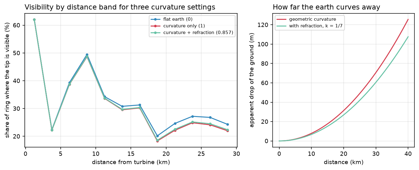
On a flat earth, a 100 m turbine on a 400 m hill would be visible for hundreds of kilometres across a plain. On the real earth, the ground curves away from a level sightline by d²/2R, where R is the earth’s radius. Refraction bends light slightly downwards and offsets about a seventh of this, so the apparent drop is (1 − k)·d²/2R with k ≈ 1/7. That is what GDAL’s default curvCoeff of 0.85714 means. Pass 0 for a flat earth and 1 for curvature without refraction.
5 km: curvature drop 2.0 m | with refraction (k=1/7) 1.7 m10 km: curvature drop 7.8 m | with refraction (k=1/7) 6.7 m20 km: curvature drop 31.4 m | with refraction (k=1/7) 26.9 m30 km: curvature drop 70.6 m | with refraction (k=1/7) 60.5 mflat earth (0) visible 802.5 km2 | 25.7% of the 20-30 km ringcurvature only (1) visible 750.3 km2 | 23.3% of the 20-30 km ringcurvature + refraction (0.857) visible 757.9 km2 | 23.6% of the 20-30 km ringAt 30 km the ground has dropped 60 m, more than half the height of the turbine. A flat-earth viewshed claims 802.5 km² instead of 757.9 km², and almost all the extra area is far away, where viewers would be looking just over a ridge. Refraction is variable (it is stronger over cold water and in temperature inversions), so treat k = 1/7 as a convention, not a measurement.
Step 6: a cumulative viewshed (ZTV) from 26 turbines
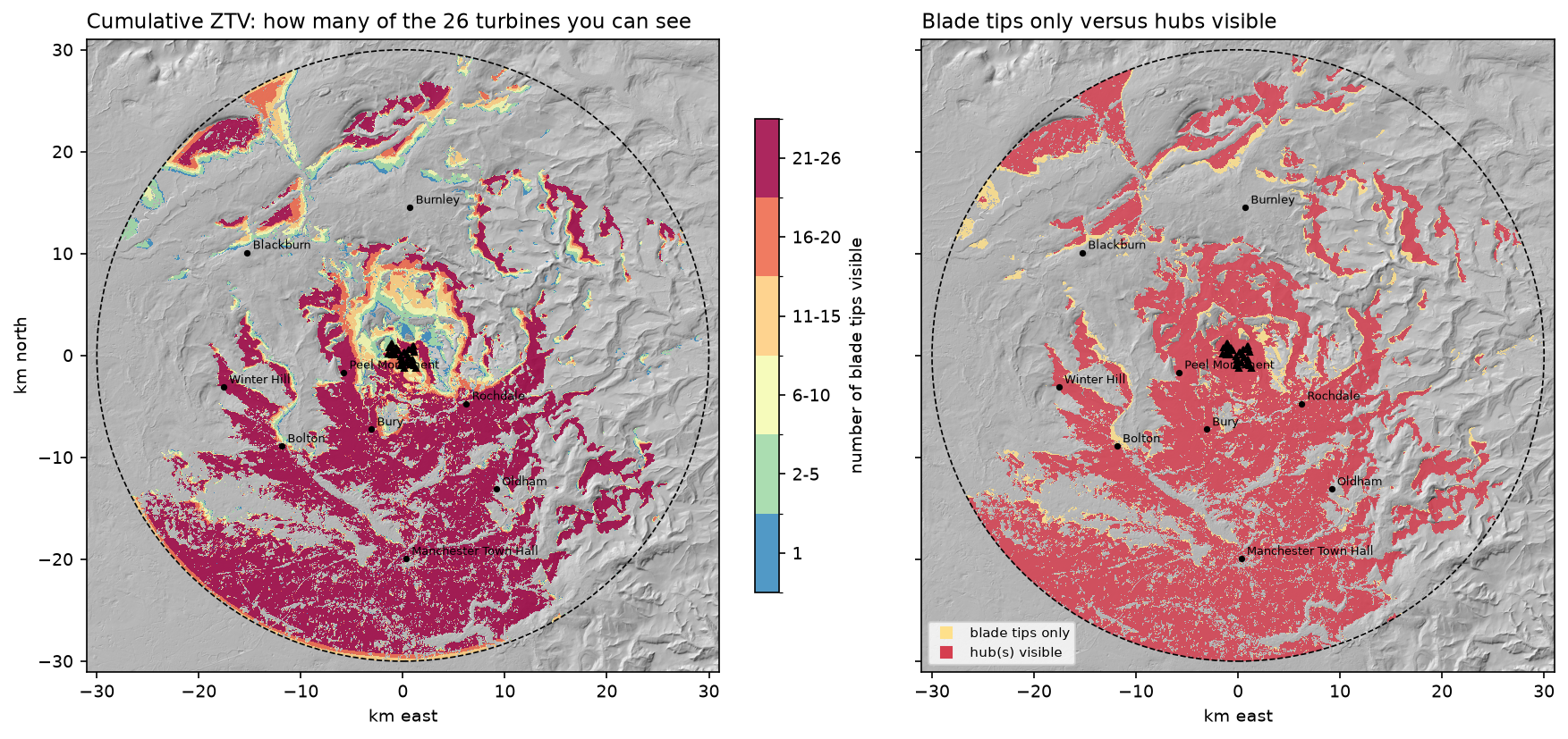
A wind farm ZTV is a cumulative viewshed: one viewshed per turbine, added up, so each cell holds the number of turbines visible from it. It is usual to compute it twice. Once for blade tips (can you see any moving part?) and once for hubs (can you see the rotor centre, a much stronger visual cue?):
n_tip = np.zeros(dem.shape, "int16"); n_hub = np.zeros(dem.shape, "int16")for x, y in zip(tx, ty): n_tip += gdal_viewshed(band, x, y, TIP_H, EYE_H) == 1 n_hub += gdal_viewshed(band, x, y, HUB_H, EYE_H) == 152 viewsheds in 2.1 sat least one blade tip 1017 km2 36.0%at least one hub 918 km2 32.5%blade tips only, no hub 99 km2 3.5%all 26 tips 504 km2 17.8%no part of any turbine 1810 km2 64.0%
turbines visible at named places (2 m eye height, GLO-30 surface):place km tips hubsManchester Town Hall 19.9 0 0Bury 7.9 25 23Rochdale 7.8 24 17Bolton 14.8 26 7Oldham 16.0 0 0Ramsbottom 4.5 13 9Edenfield 3.9 8 6Rawtenstall 5.3 0 0Burnley 14.6 0 0Blackburn 18.3 0 0Peel Monument 6.0 26 26Winter Hill 17.8 26 26Fifty-two viewsheds over 4.3 million cells take two seconds. The pattern is classic upland wind farm: the plateau edge faces south, so the farm is widely visible across the Manchester plain (Bury 25 tips, Bolton 26) but hidden from the deep Rossendale valleys to the north. Rawtenstall, 5.3 km away, sees nothing, while Bolton at 14.8 km and the summit of Winter Hill at 17.8 km see every tip. Distance is a poor guide to visibility in hilly country.
Point results need care. Manchester Town Hall and Oldham show zero, but the map shows visible ground close to both. A single 30 m cell in a town centre is sensitive to the exact location and to GLO-30’s partial building heights. The script also writes ztv_tips_count.tif and ztv_hubs_count.tif, so you can inspect them in QGIS.
Step 7: line-of-sight profiles
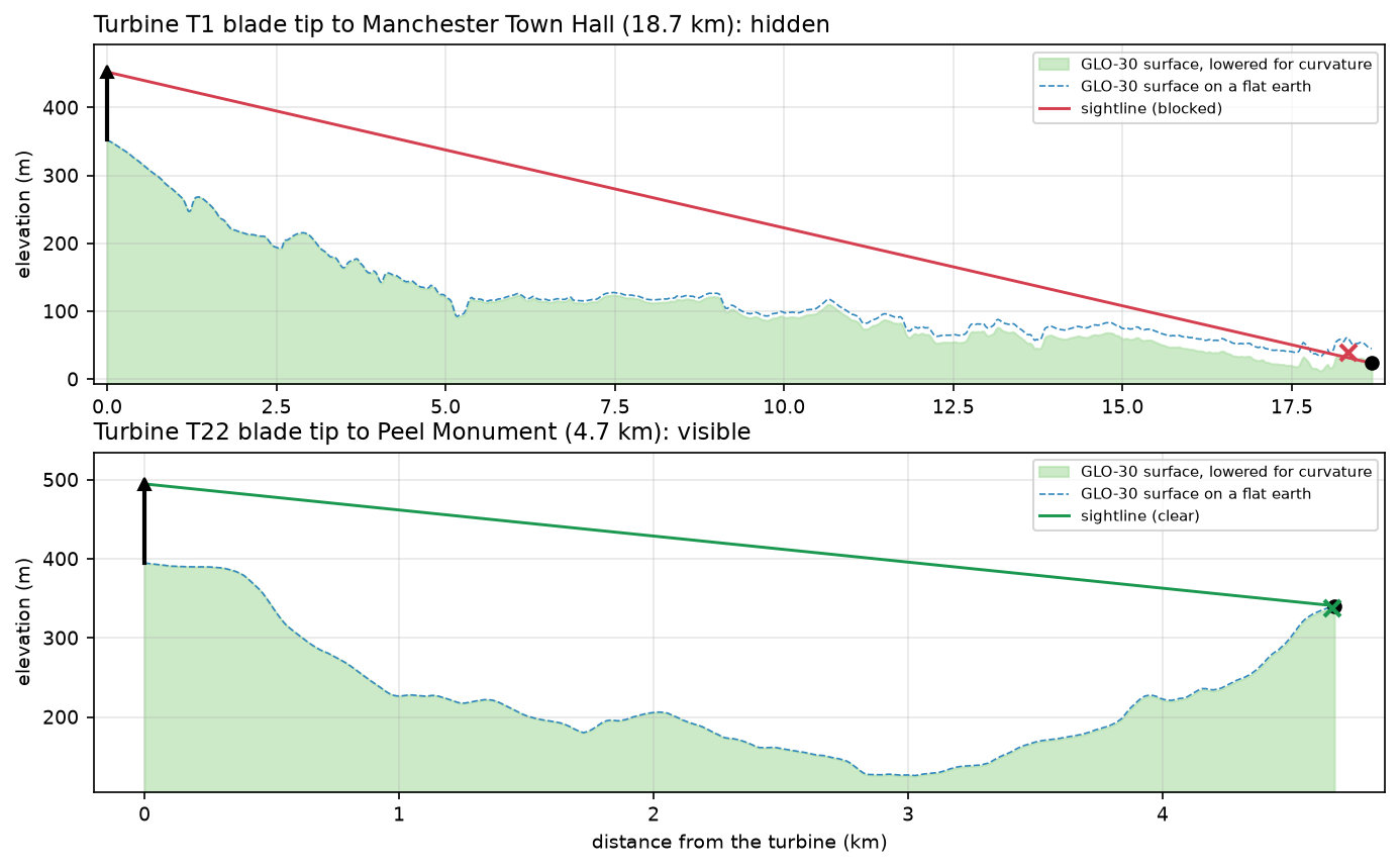
A ZTV says whether a place sees a turbine; a line-of-sight profile explains why. We sample the DEM along the straight line with bilinear interpolation every 15 m, lower it for curvature, and compare it with the sightline from the blade tip to the viewer’s eye:
def los_profile(x0, y0, x1, y1, obs_h, tgt_h, z=dem, gt=GT, curv=CURV, step=CELL / 2): """Sample the DEM along a straight line, lower it for curvature and test the sightline.""" L = np.hypot(x1 - x0, y1 - y0) d = np.arange(0, L + step, step); d[-1] = L xs, ys = x0 + (x1 - x0) * d / L, y0 + (y1 - y0) * d / L fc = (xs - gt[0]) / gt[1] - 0.5; fr = (ys - gt[3]) / gt[5] - 0.5 # bilinear sampling c0, r0 = np.floor(fc).astype(int), np.floor(fr).astype(int); fx, fy = fc - c0, fr - r0 g = (z[r0, c0] * (1 - fx) * (1 - fy) + z[r0, c0 + 1] * fx * (1 - fy) + z[r0 + 1, c0] * (1 - fx) * fy + z[r0 + 1, c0 + 1] * fx * fy) g_eff = g - curv * d ** 2 / (2 * R_EARTH) z0, z1 = g_eff[0] + obs_h, g_eff[-1] + tgt_h sight = z0 + (z1 - z0) * d / L clearance = sight[1:-1] - g_eff[1:-1] worst = int(np.argmin(clearance)) + 1 return d, g, g_eff, sight, clearance.min() >= 0, worstT1 tip -> Manchester Town Hall: 18.7 km | BLOCKED | tightest point 18.33 km from the turbine, sightline -6.8 m above the curvature-corrected ground | curvature + refraction at the viewer 23.5 mT22 tip -> Peel Monument: 4.7 km | VISIBLE | tightest point 4.67 km from the turbine, sightline +3.1 m above the curvature-corrected ground | curvature + refraction at the viewer 1.5 mThe Manchester profile is a near miss: the sightline is blocked 370 m before the viewer by 6.8 m. That is about the height of a two-storey building, and GLO-30 includes some of the city’s buildings, so this result is well within the DEM’s uncertainty. Curvature lowers the ground at the viewer by 23.5 m relative to the turbine. Peel Monument, on Holcombe Hill above Ramsbottom, looks across the Irwell valley; its tightest point is the hillside just below the viewer, which the sightline clears by 3.1 m.
Step 8: DSM versus DTM with Environment Agency LiDAR
Everything so far used a 30 m surface that only partly includes trees and buildings. To see how much they matter, we take an 8 km × 8 km window covering Ramsbottom, Edenfield and the western half of the wind farm. We download the Environment Agency’s LIDAR Composite 1 m DTM (bare earth) and first-return DSM (surface) from its WCS, one 1 km tile at a time, and resample both to 2 m:
EA_WCS = { "dtm": ("lidar-composite-digital-terrain-model-dtm-1m", "13787b9a-26a4-4775-8523-806d13af58fc__Lidar_Composite_Elevation_DTM_1m"), "dsm": ("lidar-composite-digital-surface-model-first-return-dsm-1m", "df4e3ec3-315e-48aa-aaaf-b5ae74d7b2bb__Lidar_Composite_Elevation_FZ_DSM_1m"),}url = (f"https://environment.data.gov.uk/spatialdata/{service}/wcs?service=WCS&version=2.0.1" f"&request=GetCoverage&CoverageId={cov}&format=image/tiff" f"&subset=E({x0},{x0 + 1000})&subset=N({y0},{y0 + 1000})")Two problems need handling before a fair comparison:
- The turbines are in the DSM. LiDAR records the towers as 60 m spikes. Left in, the observer would stand on top of the tower, so we reset the DSM to the DTM within 12 m of each turbine.
- On a DSM, the viewer would stand on the roof or in the treetop. A person stands on the ground, among the trees. GDAL handles this with
heightMode=gdal.GVOT_MIN_TARGET_HEIGHT_FROM_DEM, which returns, for every cell, the lowest elevation a target must reach to be seen over the DSM. A ground-level viewer sees the turbine if DTM + 2 m reaches that elevation.
for x, y in local_turb: n_dtm += gdal_viewshed(dtm_ds.GetRasterBand(1), x, y, TIP_H, EYE_H, max_dist=15_000, shape=dtm.shape, gt=LGT) == 1 # lowest elevation a target in each cell must reach to be seen over the DSM; a ground-level eye is at DTM + 2 m need = gdal_viewshed(dsm_ds.GetRasterBand(1), x, y, TIP_H, 0, max_dist=15_000, shape=dtm.shape, gt=LGT, height_mode=gdal.GVOT_MIN_TARGET_HEIGHT_FROM_DEM) n_dsm += np.nan_to_num(need <= dtm + EYE_H, nan=0).astype("int16")grid 4000 x 4000 cells of 2 m | no data: DTM 0.00%, DSM 0.00%turbines inside the LiDAR window: 26 of 26DSM - DTM within 12 m of each turbine (the tower in the DSM): median 60.1 m, max 65.7 m; reset to the DTMcells more than 2.5 m above ground (trees, buildings): 9.3%52 LiDAR viewsheds in 10.9 sall cells : >=1 tip visible on DTM 81.7% | on DSM 64.7% | mean tips visible 11.6 vs 8.8open ground only : >=1 tip visible on DTM 83.1% | on DSM 73.5% | mean tips visible 11.9 vs 10.0Edenfield 1 km2 around (379868, 419380): >=1 tip visible on DTM 90.7% | on DSM (at ground level) 52.6%Ramsbottom 1 km2 around (379169, 416835): >=1 tip visible on DTM 90.7% | on DSM (at ground level) 29.0%The LiDAR measures the towers at a median of 60.1 m, exactly the published hub height, which is a good check that the data are aligned. Only 9.3% of the window is more than 2.5 m above ground, mostly moorland. Even so, surface objects remove a fifth of the visible area: 81.7% falls to 64.7%.
The effect is concentrated where people live. In the square kilometre around Ramsbottom, a bare-earth ZTV says 90.7% of the ground sees a turbine tip. Standing in the streets among the buildings and trees, only 29.0% does. Even in open fields (cells less than 1 m above the DTM), visibility drops from 83.1% to 73.5%, because hedgerows and woods block the view. Both town squares show 90.7% on the DTM at different locations, which is a coincidence.
DSM or DTM: which should you use?
| Question | Use |
|---|---|
| Statutory wind farm or mast ZTV in the UK | Bare-earth DTM, as a worst case. Landscape guidance treats the ZTV as theoretical and adds screening in the field and in photomontages. |
| Realistic visibility for residents or walkers | DSM for blockers, DTM + eye height for the viewer, as in Step 8. |
| Telecoms line of sight | DSM, plus clearance of the Fresnel zone, not just the sightline. |
| Viewpoint from a summit or tower | DSM if the summit is wooded or the view is over a town; a DTM is fine for open mountain tops. |
| Global studies at 30 m | Copernicus GLO-30, remembering it is a partial DSM. |
A DSM is a snapshot. Deciduous trees in winter block much less than the leaf-on LiDAR suggests, and trees grow or are felled. A DTM viewshed is reproducible and conservative, which is why planning work uses it as the baseline.
Pitfalls and limitations
- Resolution. At 30 m, a ridge, embankment or row of houses may disappear between cells. Fringes of the viewshed are uncertain by at least one cell, as the 98.5% agreement between two correct algorithms shows.
- Vertical accuracy. GLO-30’s absolute vertical error is a few metres in open terrain and worse in towns and forests. A 6.8 m miss on the Manchester profile is within that uncertainty.
- Reciprocity is approximate. Swapping observer and target is exact for a single straight line. On a grid, the paths and interpolation differ slightly, so “turbine sees cell” and “cell sees turbine” can disagree at the edges.
- Blade-tip assumption. A tip ZTV counts a cell as visible if any part of the rotor’s highest point could be seen. A blade tip just above a ridge at 25 km is barely perceptible; a hub ZTV and a distance band give a more honest picture.
- What is not modelled: atmospheric visibility, lighting and contrast, the angle the turbine subtends, and screening by walls and windows.
- Projection. Run viewsheds in a projected CRS with square metric cells. In degrees, distances and cell sizes are wrong, and GDAL’s curvature correction becomes meaningless.
Frequently asked questions
How do you calculate a viewshed in Python?
Use GDAL’s Python bindings: open the DEM, get the band and call gdal.ViewshedGenerate with the observer’s map coordinates, observer height, target height and maximum distance. It returns a raster where visible cells hold 1. For more control, write a ray-casting algorithm in numpy (Step 4) or use the viewshed functions in packages such as xarray-spatial. In QGIS, the Visibility Analysis plugin and the GDAL Viewshed tool in the Processing toolbox do the same job.
What is the difference between a viewshed and line of sight?
A line of sight tests one pair of points: can A see B? A viewshed tests one point against every cell of a DEM and returns a map. Both use the same test, whether the straight sightline stays above the terrain. A line-of-sight profile is useful to explain a viewshed result, such as which ridge blocks a view.
Should a viewshed account for earth curvature?
Yes, beyond about 5 km. The ground drops 2 m below a level line at 5 km, 7.8 m at 10 km and 70.6 m at 30 km. Atmospheric refraction bends light back by about a seventh of that, so most tools use a coefficient of 0.857 (1 − 1/7). In this tutorial, ignoring curvature overstated one turbine’s visible area by 6%, nearly all of it far away.
What is a zone of theoretical visibility (ZTV)?
A ZTV is a map of where a development such as a wind farm could in theory be seen, computed from terrain alone. For wind farms it is a cumulative viewshed of all turbines, usually shown as the number of hubs or blade tips visible, within a radius that depends on turbine height. It is “theoretical” because it ignores trees, buildings and atmospheric conditions, so it overstates actual visibility.
Should I use a DSM or a DTM for a viewshed?
Use a DTM for a conservative, reproducible baseline, such as a planning ZTV. Use a DSM when you need realistic visibility, but keep the viewer on the ground (DTM + eye height) and use the DSM only for what blocks the view. In this tutorial, adding trees and buildings from LiDAR cut the area that could see a turbine from 81.7% to 64.7%, and in Ramsbottom from 90.7% to 29.0%.
Which DEM is best for viewshed analysis?
Use the most detailed DEM that covers your area. In England, the Environment Agency’s 1 m LiDAR DTM and DSM are free. Other UK nations and many countries have national LiDAR too (see UK data sources). For larger areas or other countries, Copernicus GLO-30 is the best free global DEM, but it is a partial surface model. SRTM is older and noisier.
Next steps
- Compute slope, aspect and hillshade from the same kind of DEM with raster terrain analysis in Python with rasterio.
- Use LiDAR DSMs for something else that depends on what blocks the sky: rooftop solar potential from LiDAR in Python uses horizon angles, a close cousin of the viewshed, to shade every roof.
- Work with the point clouds behind DTMs and DSMs in LiDAR point clouds in Python with laspy, and get heights for individual buildings in building footprints and heights from LiDAR.
- Measure the trees that block views with a canopy height map in Python.
- Turn the DEM into a physical model with DEM to STL in Python, or route water over it with watershed delineation in Python.
- Summarise the ZTV by parish or ward with zonal statistics in Python.
Data and licences
- Copernicus DEM GLO-30: © DLR e.V. 2010–2014 and © Airbus Defence and Space GmbH 2014–2018, provided under COPERNICUS by the European Union and ESA; all rights reserved. Free to use under the Copernicus DEM licence. Accessed from the Microsoft Planetary Computer on 23 October 2026.
- LiDAR: Environment Agency LIDAR Composite DTM and first-return DSM, 1 m. © Environment Agency copyright and/or database right 2026. All rights reserved. Available under the Open Government Licence v3.0. Accessed from the Environment Agency WCS on 23 October 2026.
- Turbine positions: © OpenStreetMap contributors, available under the Open Database Licence (ODbL). Accessed via the Overpass API on 23 October 2026.
- Code:
viewshed_analysis.py, tested with Python 3.12.0, GDAL 3.13.3, numpy 2.5.4, requests 2.34.2, pystac-client 0.9.0, planetary-computer 1.0.0 and matplotlib 3.11.2.
Key terms
- Viewshed
- The set of raster cells visible from an observer point at a given height, for a target at a given height above the surface. A cell is visible if the straight sightline between them never passes below the terrain.
- ZTV
- Zone of theoretical visibility: the area from which a development such as a wind farm could in theory be seen, computed from terrain alone. Used in landscape and visual impact assessment (LVIA) in the UK.
- Cumulative viewshed
- The sum of several viewsheds, so each cell holds the number of observers (here turbines) that can see it, or that it can see.
- DSM and DTM
- A digital surface model includes buildings, trees and other objects on the ground; a digital terrain model is the bare earth with them removed. Copernicus GLO-30 is a radar DSM; LiDAR gives both.
- Refraction coefficient
- The fraction by which the atmosphere bends light back towards the ground, partly offsetting earth curvature. 1/7 (0.143) is the usual value for visible light; GDAL's default curvature coefficient 0.85714 is 1 − 1/7.
- Line-of-sight profile
- A cross-section of the terrain between two points with the straight sightline drawn on top. Where the line dips below the ground, the view is blocked.
Data for this tutorial
- Copernicus DEM (GLO-30 / GLO-90) · 30 m global DSM, read as GLO-30 from the Planetary Computer
- Microsoft Planetary Computer · The cop-dem-glo-30 collection, streamed as COGs
- Environment Agency National LIDAR Programme · LIDAR Composite 1 m DTM and first-return DSM for England, via WCS
- OpenStreetMap · Positions of the 26 Scout Moor wind turbines, via the Overpass API
Licences and formats for each source are listed in the GIS data sources catalogue.