Canopy height map in Python: Meta 1 m and ETH 10 m maps checked against UK LiDAR (Forest of Dean)
Read the open Meta/WRI global 1 m canopy height map from AWS with no login, compare it with ETH Global Canopy Height 2020, and validate both against a canopy height model made from Environment Agency LiDAR in the Forest of Dean: CRS alignment, bias, RMSE, hexbin plots, height classes and honest limitations.
- Level
- Intermediate
- Tested with
- Python 3.12
- Source code
- Download scripts
Key takeaways
- Meta and WRI's global canopy height map is a free 1 m product on AWS open data. Find the zoom-9 QuadKey tile in tiles.geojson and read a window of chm/<quadkey>.tif with rasterio; no login or download tool is needed.
- The tile is in Web Mercator (EPSG:3857), so its 1.19 m pixels are only 0.74 m on the ground in the Forest of Dean. Reproject everything onto one British National Grid grid before you compare a single pixel.
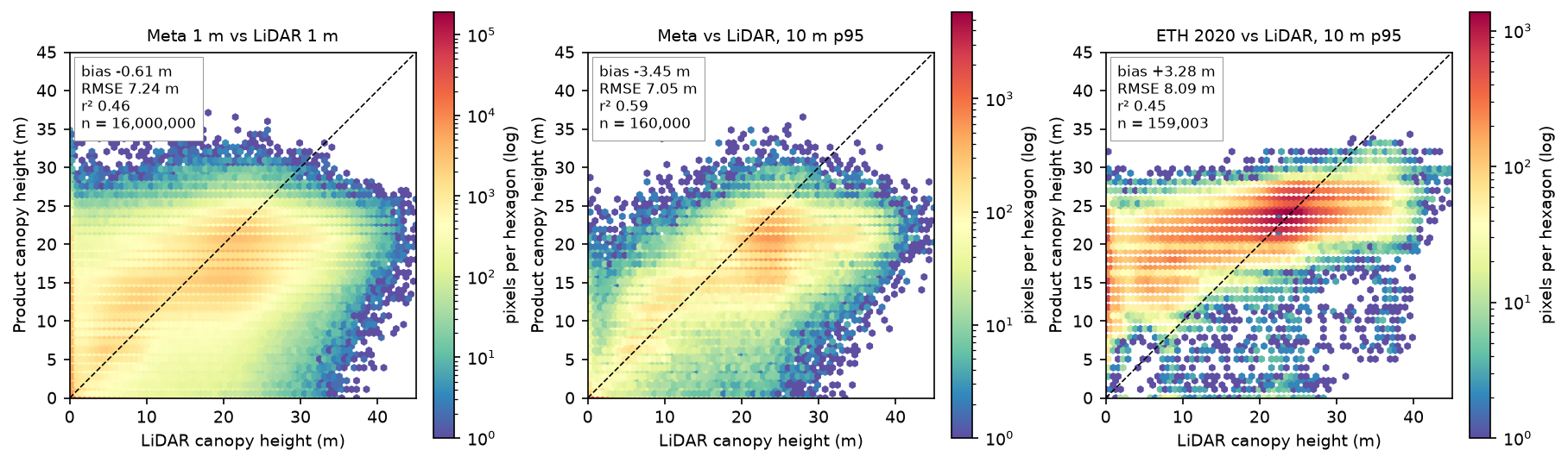
- Against an Environment Agency LiDAR canopy height model over 1,600 ha of the Forest of Dean, Meta's 1 m heights have a bias of −0.61 m and an RMSE of 7.24 m (r² 0.46). At 10 m the RMSE falls to 5.57 m for mean heights.
- Both global maps saturate. Where the LiDAR canopy is 30–35 m tall, Meta reads 13.1 m too low and ETH 7.1 m too low; ETH also puts 15 m of canopy on open ground and stretches 20–30 m forest across 1,219 ha, against 416 ha in the LiDAR.
- The maps are useful for where the forest is and roughly how tall, not for the height of a given tree. Different epochs, leaf-off LiDAR, edge effects and a 5 m shift all inflate the errors, and you should report them.
Before you start
- Comfortable with NumPy arrays and reading rasters with rasterio (the raster terrain analysis tutorial is a good primer)
- Python 3.10+ with rasterio, numpy, scipy, pandas, shapely, requests and matplotlib
- An internet connection: the Meta map is on AWS open data, the ETH map on an ETH Zurich file share and the LiDAR on an Environment Agency web service, and none needs an account
Short answer: to make a canopy height map in Python without collecting any data, read the Meta/WRI High Resolution Canopy Height Map. It is a free, global 1 m map on AWS open data. Find your tile’s QuadKey in tiles.geojson, open chm/<quadkey>.tif with rasterio.open("/vsicurl/" + url) and read only the window you need. Heights are whole metres in a uint8 band, in Web Mercator. Reproject them onto a local grid, such as the British National Grid, before you do anything else. Then check them against LiDAR if you can. In the Forest of Dean, Meta’s map gets the pattern of the forest right (r² 0.59 at 10 m), but it reads tall stands 9–17 m too low, and the ETH 10 m map is no better.
Global canopy height maps made from satellite imagery and machine learning appeared from 2022 onwards. They promise tree heights everywhere, for carbon accounting, habitat mapping and forest monitoring. But how good are they on a real British forest? We test two of them in the Forest of Dean, Gloucestershire: a 4 km × 4 km block around the Cannop Valley with oak and beech high forest, conifer plantations of every age and fresh clear-fells. The reference is a canopy height model from the Environment Agency’s 1 m LiDAR, which is free and open in England.
You will learn how to:
- find and read the right tile of the Meta canopy height map straight from AWS;
- read a window of the ETH Global Canopy Height 2020 map, a 10 m alternative;
- build a LiDAR canopy height model from the Environment Agency’s DSM and DTM, and fill its pits;
- put three products in three different CRSs onto one British National Grid grid, and check the co-registration;
- compare them pixel by pixel, with bias, RMSE, r² and hexbin plots;
- measure saturation in tall canopy and edge effects around gaps;
- turn the heights into height-class maps and areas.
The full script is canopy_height.py. It caches everything it downloads in a data/ folder, about 120 MB in total, and writes figures, GeoTIFFs and CSV tables to output/.
The three canopy height products
| Meta/WRI canopy height | ETH Global Canopy Height | Environment Agency LiDAR | |
|---|---|---|---|
| What it is | Vision transformer applied to Maxar imagery, trained on aerial LiDAR and corrected with GEDI | Deep learning on Sentinel-2, trained on GEDI spaceborne LiDAR | Airborne laser scanning, first-return DSM minus DTM |
| Resolution | about 1 m (1.19 m Web Mercator pixels) | 10 m (1/12,000 degree) | 1 m |
| Epoch | imagery mostly 2018–2020 (2018-05-14 here) | 2020 | composite of surveys from November 2016 to May 2022, flown leaf-off |
| Format | 65,536 × 65,536 uint8 GeoTIFF per QuadKey tile, EPSG:3857 |
3° × 3° Cloud Optimised GeoTIFFs, EPSG:4326 | WCS 2.0.1, float32, EPSG:27700 |
| Access | public S3 bucket, no login | public file share, no login | public web service, no key |
| Licence | CC BY 4.0 | CC BY 4.0 | Open Government Licence v3.0 |
Both global maps predict roughly the top of the canopy: Meta’s model was trained on LiDAR canopy height at 1 m, and ETH’s on the GEDI RH98 metric, which is close to the 95th–98th percentile of canopy height in a 25 m footprint. That matters when we choose what to compare them with.
Step 1: find and read the Meta canopy height tile
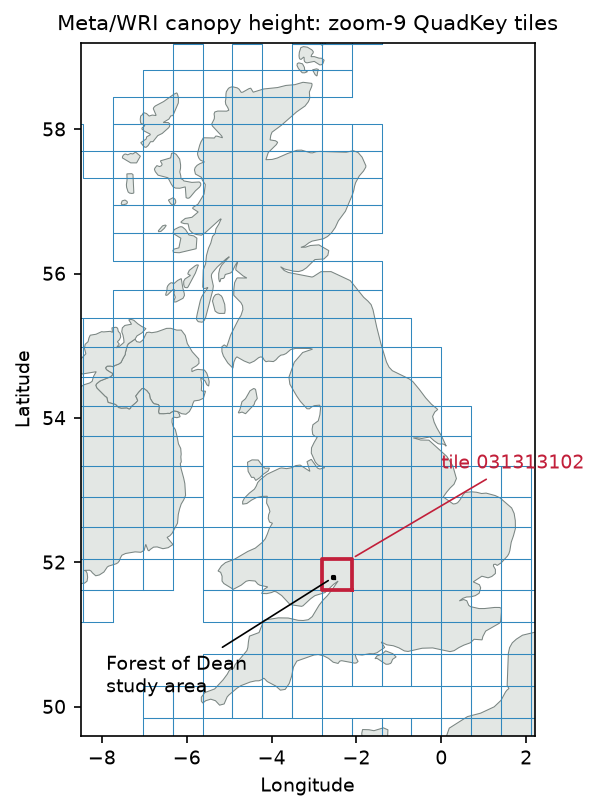
The map lives under s3://dataforgood-fb-data/forests/v1/alsgedi_global_v6_float/, which you can reach over plain HTTPS. A tiles.geojson index lists every tile as a zoom-9 Web Mercator QuadKey. We intersect it with our area, and confirm the answer with a ten-line QuadKey function:
META_ROOT = "https://dataforgood-fb-data.s3.amazonaws.com/forests/v1/alsgedi_global_v6_float"AOI_BNG = (360000, 209000, 364000, 213000)          # xmin, ymin, xmax, ymax in EPSG:27700

def quadkey(lon, lat, zoom):    """Bing/Web Mercator QuadKey of the tile that contains a point."""    n = 2 ** zoom    x = int((lon + 180) / 360 * n)    lat_r = np.radians(lat)    y = int((1 - np.log(np.tan(lat_r) + 1 / np.cos(lat_r)) / np.pi) / 2 * n)    digits = []    for i in range(zoom, 0, -1):        mask = 1 << (i - 1)        digits.append(str((1 if x & mask else 0) + (2 if y & mask else 0)))    return "".join(digits)

tiles = json.loads(tiles_path.read_text())["features"]   # downloaded once from META_ROOT/tiles.geojsonaoi_ll = transform_bounds(BNG, "EPSG:4326", *AOI_BNG)aoi_poly = box(*aoi_ll)hits = [f["properties"]["tile"] for f in tiles if shape(f["geometry"]).intersects(aoi_poly)]TILE = hits[0]meta_url = f"{META_ROOT}/chm/{TILE}.tif"
with rasterio.open("/vsicurl/" + meta_url) as src: b3857 = transform_bounds(BNG, src.crs, *AOI_BNG) pad = 60 win = from_bounds(b3857[0] - pad, b3857[1] - pad, b3857[2] + pad, b3857[3] + pad, src.transform).round_offsets().round_lengths() meta_3857 = src.read(1, window=win) meta_3857_tf = src.window_transform(win)56,145 tiles in the global index (zoom-9 QuadKeys)AOI lon/lat bounds: -2.5817, 51.7782, -2.5232, 51.8145tiles intersecting the AOI: ['031313102']; QuadKey computed from the AOI centre: 031313102chm/031313102.tif: 65536 x 65536 px, uint8, pixel 1.1943 m, tiled=False, block (1, 65536), nodata=NoneCRS: EPSG:3857 (Web Mercator); origin x -313086.1, y 6809622.0read window 5547 x 5561 px; heights 0..37 mWeb Mercator pixel 1.194 m on the map = 0.739 m on the ground at 51.80 Nimagery dates in tile 031313102: 13 footprints, 2017-05-07 .. 2018-10-10imagery date(s) under the AOI: ['2018-05-14']Three details in that output matter later:
- The pixel is smaller than it looks. Web Mercator stretches distances by 1/cos(latitude), so a 1.19 m map pixel is 0.74 m on the ground at 51.8°N. Never compute areas by counting pixels in EPSG:3857.
- Heights are whole metres from 0 to 37 m in this window, with no nodata value. A zero means “no canopy”, not “missing”.
- The imagery under our area was taken on 14 May 2018. The
metadata/<quadkey>.geojsonfile gives the acquisition date of each image footprint, and you should always look it up: one tile mixes 13 images from 2017 and 2018.
Step 2: read the ETH Global Canopy Height 2020 map
The ETH map by Lang et al. (2023) is the best known alternative. It is a 10 m map for 2020, made from Sentinel-2 and trained on GEDI. The 3° × 3° tiles are Cloud Optimised GeoTIFFs on an ETH Zurich file share. That server does not answer the HEAD requests that GDAL sends first, so we tell /vsicurl to skip them:
ETH_URL = ("https://libdrive.ethz.ch/index.php/s/cO8or7iOe5dT2Rt/download?path=%2F3deg_cogs" "&files=ETH_GlobalCanopyHeight_10m_2020_N51W003_Map.tif")eth_vsi = "/vsicurl?use_head=no&max_retry=3&url=" + urllib.parse.quote(ETH_URL, safe="")with rasterio.Env(GDAL_DISABLE_READDIR_ON_OPEN="EMPTY_DIR"): with rasterio.open(eth_vsi) as src: d = 0.002 w = from_bounds(aoi_ll[0] - d, aoi_ll[1] - d, aoi_ll[2] + d, aoi_ll[3] + d, src.transform).round_offsets().round_lengths() eth_ll = src.read(1, window=w) eth_tf, eth_crs, eth_nd = src.window_transform(w), src.crs, src.nodataN51W003 tile: 36000 x 36000 px of 0.00008333 deg, EPSG:4326, nodata=255.0, overviews [2, 4, 8, 16, 32, 64]ETH pixel on the ground: 5.7 m east-west x 9.3 m north-southThe tile is named after its south-west corner (51°N, 3°W). Because it is on a latitude–longitude grid, its “10 m” pixels are 5.7 m by 9.3 m in Britain. Heights are again whole metres, with 255 as nodata.
Step 3: a LiDAR canopy height model from Environment Agency data
The Environment Agency publishes its LiDAR Composite 1 m DTM and first-return DSM for England through open Web Coverage Services. A GetCoverage request returns a GeoTIFF for any box in British National Grid metres, with no API key. We ask for 1 km tiles and paste them into one 4,000 × 4,000 array:
EA_WCS = {    "dtm": ("lidar-composite-digital-terrain-model-dtm-1m",            "13787b9a-26a4-4775-8523-806d13af58fc__Lidar_Composite_Elevation_DTM_1m"),    "dsm": ("lidar-composite-digital-surface-model-first-return-dsm-1m",            "df4e3ec3-315e-48aa-aaaf-b5ae74d7b2bb__Lidar_Composite_Elevation_FZ_DSM_1m"),}

def ea_wcs(product, x0, y0, size=1000):    """One 1 km x 1 km GeoTIFF from the Environment Agency WCS (no key needed)."""    service, cov = EA_WCS[product]    url = (f"https://environment.data.gov.uk/spatialdata/{service}/wcs?service=WCS&version=2.0.1"           f"&request=GetCoverage&CoverageId={cov}&format=image/tiff"           f"&subset=E({x0},{x0 + size})&subset=N({y0},{y0 + size})")    r = requests.get(url, timeout=180)    r.raise_for_status()    return r.content

dtm, grid_tf = ea_mosaic("dtm") # 16 tiles each, pasted by their top-left cornerdsm, _ = ea_mosaic("dsm")chm = dsm - dtmchm[chm < 0] = 0chm[chm > 50] = np.nan # isolated spikes (birds, power lines) are not treeschm_raw = chm.copy()# Leaf-off first returns pass through gaps in broadleaf crowns and leave "pits"; a 3 x 3 grey closing fills themchm = ndimage.grey_closing(np.nan_to_num(chm_raw), size=(3, 3)).astype("float32")chm[np.isnan(chm_raw)] = np.nanone WCS tile: 1000 x 1000 px, float32, EPSG:27700, nodata -3.4e+38grid: 4000 x 4000 px of 1 m, origin E 360000 N 213000DTM 51.0..200.0 m; DSM 51.2..237.6 m; no data: 0.00%raw DSM - DTM: min -1.46 m, max 49.09 m, 0.00% below -0.5 m, 0 px above 50 mpits: in 10 m cells whose p95 is >= 15 m, 13.2% of 1 m pixels are < 2 m before pit filling and 7.4% afterpit-filled LiDAR CHM: mean 12.98 m, canopy >= 2 m on 78.3% of the AOI, p95 28.3 m, p99 33.5 m, max 49.1 mThe composite has no gaps here, and the CHM is clean: no negative heights worth worrying about and no spikes above 50 m. The tallest tree is 49.1 m, which is plausible for the mature conifers, such as Douglas fir, planted in the Forest of Dean.
The one real problem is pits. The composite was flown in winter, when the oaks and beeches have no leaves, so many first returns came from branches or the ground beneath the crowns. Inside tall stands, 13.2% of the 1 m pixels read below 2 m. A 3 × 3 greyscale closing (a dilation followed by an erosion) fills holes narrower than about 3 m and leaves real gaps alone; it cuts the pits to 7.4% and raises the canopy share from 71.9% to 78.3%. We use the pit-filled CHM as the reference from here on and keep the raw one for comparison.
If you prefer to start from the point cloud, the LiDAR point clouds with laspy tutorial builds a DTM, DSM and CHM from raw LAZ files, which also lets you choose how to handle the pits.
Step 4: CRS alignment on the British National Grid
We now have three rasters on three grids: Web Mercator at 1.19 m, latitude–longitude at 1/12,000°, and British National Grid at 1 m. All comparisons happen on the LiDAR grid. Meta goes onto the 1 m grid with average resampling, because its pixels are smaller on the ground than the 1 m target. ETH goes onto a 10 m grid with nearest, so that its values stay as published. For the 10 m comparisons we also summarise each 10 × 10 block of the 1 m rasters by its mean and its 95th percentile:
meta = np.full(chm.shape, np.nan, "float32")reproject(meta_3857.astype("float32"), meta, src_transform=meta_3857_tf, src_crs=meta_crs,          dst_transform=grid_tf, dst_crs=BNG, dst_nodata=np.nan, resampling=Resampling.average)
grid10_tf = from_origin(AOI_BNG[0], AOI_BNG[3], 10, 10)eth = np.full((400, 400), np.nan, "float32")eth_src = eth_ll.astype("float32")eth_src[eth_ll == eth_nd] = np.nanreproject(eth_src, eth, src_transform=eth_tf, src_crs=eth_crs, src_nodata=np.nan,          dst_transform=grid10_tf, dst_crs=BNG, dst_nodata=np.nan, resampling=Resampling.nearest)

def block(a, k=10):    """Reshape a 1 m array into k x k blocks so each 10 m cell can be summarised."""    h, w = a.shape[0] // k, a.shape[1] // k    return a.reshape(h, k, w, k).swapaxes(1, 2).reshape(h, w, k * k)

lid10_mean = np.nanmean(block(chm), axis=2)lid10_p95 = np.nanpercentile(block(chm), 95, axis=2)meta10_mean = np.nanmean(block(meta), axis=2)meta10_p95 = np.nanpercentile(block(meta), 95, axis=2)
Before comparing pixels, check that the products line up. We shift the Meta grid up to 10 m in each direction and record the RMSE against the LiDAR CHM at each offset:
inner = (slice(20, -20), slice(20, -20))ref = chm[inner][::2, ::2]shift_rmse = {}for dy in range(-10, 11): for dx in range(-10, 11): shifted = np.roll(meta, (dy, dx), axis=(0, 1))[inner][::2, ::2] ok = ~np.isnan(ref) & ~np.isnan(shifted) shift_rmse[(dx, dy)] = float(np.sqrt(np.mean((shifted[ok] - ref[ok]) ** 2)))best = min(shift_rmse, key=shift_rmse.get)Meta resampled to 1 m BNG (average): (4000, 4000), NaN 0.00%ETH resampled to 10 m BNG (nearest): (400, 400), NaN 0.62%co-registration: RMSE 7.23 m as aligned; lowest 6.77 m when Meta is moved +0 m east and -5 m north (positive = east/north)The best fit comes with Meta moved 5 m south. That is not a CRS mistake: the transformation is correct, and roads and rides line up. It is most likely relief displacement. Satellite images are taken slightly off-nadir and orthorectified to the ground, not to the treetops, so the crowns of 25 m trees lean a few metres away from the satellite. We report results without the shift, because a user of the map would not know it, but this alone is worth about 0.5 m of RMSE.
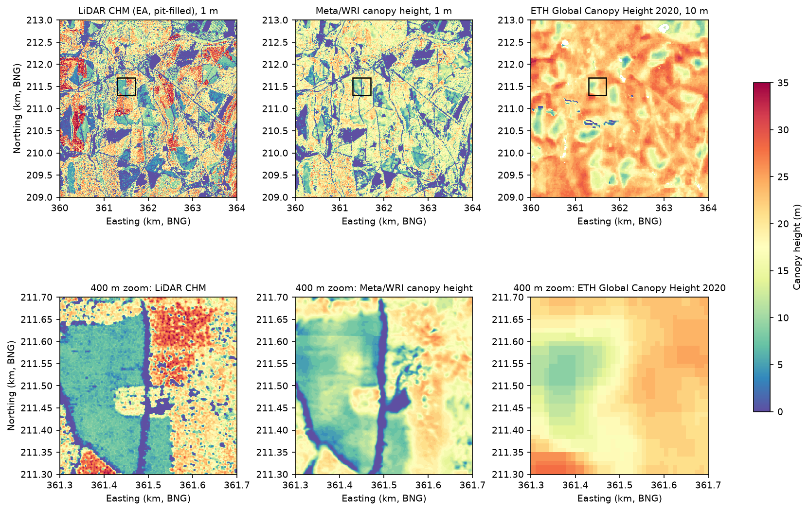
Step 5: pixel-wise comparison with the LiDAR CHM
A small function computes the usual accuracy statistics on the pixels where both rasters have data. Bias is the mean of product minus LiDAR, so a negative value means the product is too low:
def stats(pred, obs, label, subset=None):    ok = ~np.isnan(pred) & ~np.isnan(obs)    if subset is not None:        ok &= subset    p, o = pred[ok].astype("float64"), obs[ok].astype("float64")    e = p - o    r = np.corrcoef(p, o)[0, 1]    return {"comparison": label, "n": int(ok.sum()), "bias_m": e.mean(), "mae_m": np.abs(e).mean(),            "rmse_m": np.sqrt((e ** 2).mean()), "r2": r ** 2,            "mean_lidar_m": o.mean(), "mean_product_m": p.mean()}

rows = [ stats(meta, chm, "Meta 1 m vs LiDAR 1 m"), stats(meta, chm_raw, "Meta 1 m vs LiDAR 1 m, no pit filling"), stats(meta, chm, "Meta 1 m vs LiDAR 1 m, LiDAR >= 5 m", chm >= 5), stats(meta10_mean, lid10_mean, "Meta 10 m mean vs LiDAR 10 m mean"), stats(meta10_p95, lid10_p95, "Meta 10 m p95 vs LiDAR 10 m p95"), stats(eth, lid10_p95, "ETH 10 m vs LiDAR 10 m p95"), stats(meta10_p95, lid10_p95, "Meta 10 m p95 vs LiDAR p95, LiDAR >= 5 m", lid10_p95 >= 5), stats(eth, lid10_p95, "ETH 10 m vs LiDAR p95, LiDAR >= 5 m", lid10_p95 >= 5),] comparison n bias_m mae_m rmse_m r2 mean_lidar_m mean_product_m Meta 1 m vs LiDAR 1 m 16000000 -0.61 5.30 7.24 0.46 12.98 12.37 Meta 1 m vs LiDAR 1 m, no pit filling 16000000 1.12 6.05 8.15 0.35 11.25 12.37 Meta 1 m vs LiDAR 1 m, LiDAR >= 5 m 11415934 -2.42 5.67 7.26 0.21 17.74 15.32 Meta 10 m mean vs LiDAR 10 m mean 160000 -0.61 4.17 5.57 0.59 12.98 12.37 Meta 10 m p95 vs LiDAR 10 m p95 160000 -3.45 5.34 7.05 0.59 18.47 15.02 ETH 10 m vs LiDAR 10 m p95 159003 3.28 6.17 8.09 0.45 18.57 21.85Meta 10 m p95 vs LiDAR p95, LiDAR >= 5 m 139874 -4.10 5.80 7.40 0.37 20.92 16.82 ETH 10 m vs LiDAR p95, LiDAR >= 5 m 139683 1.71 5.00 6.49 0.33 20.93 22.64What the table says:
- At 1 m, Meta is unbiased on average but noisy. The bias is only −0.61 m, but the RMSE is 7.24 m and r² 0.46. Pixel-level errors of this size are normal for 1 m comparisons: a crown edge a metre out of place produces a 20 m error in one pixel.
- The reference matters. Against the raw CHM, without pit filling, Meta seems to overestimate by 1.12 m and the RMSE rises to 8.15 m. A leaf-off LiDAR CHM is not the “truth” without some care.
- Aggregating helps. At 10 m, Meta’s mean height has an RMSE of 5.57 m and r² 0.59. Comparing the top of the canopy (p95), Meta is 3.45 m too low.
- ETH is too high on average (+3.28 m against the LiDAR p95) and has the largest RMSE, 8.09 m. Restricted to forest (LiDAR p95 of at least 5 m), its RMSE drops to 6.49 m and its bias to +1.71 m: much of its error is on open ground.
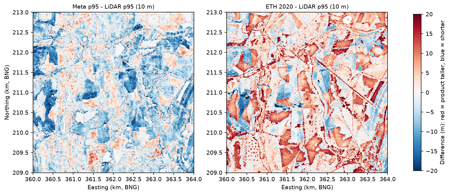
The ETH difference map shows whole compartments, with straight forestry boundaries, that ETH makes 10–20 m taller than the LiDAR. In many of them Meta, from 2018 imagery, agrees with the LiDAR that the canopy is low. These are mostly young plantations and restocked clear-fells. At 10 m resolution, a dense young crop of 4–8 m trees looks much like mature forest, and the model maps them to typical forest heights.
Step 6: saturation of tall canopy and edge effects
Two kinds of error are well known for image-based canopy height models. Saturation means the model cannot tell a 25 m stand from a 40 m one. Edge effects mean heights bleed across the boundary between tall canopy and open ground. We measure both. For saturation, we bin the pixels by LiDAR height:
bins = [0, 2, 5, 10, 15, 20, 25, 30, 35, 50]labels = [f"{a}-{b}" for a, b in zip(bins[:-1], bins[1:])]for name, pred, obs in [("Meta 1 m", meta, chm), ("Meta 10 m p95", meta10_p95, lid10_p95), ("ETH 10 m", eth, lid10_p95)]: ok = ~np.isnan(pred) & ~np.isnan(obs) p, o = pred[ok], obs[ok] idx = np.digitize(o, bins) - 1 # ... mean, quartiles and bias of p - o for each binmean product - LiDAR (m) by LiDAR height bin:product ETH 10 m Meta 1 m Meta 10 m p95lidar_bin_m0-2 +15.14 +3.61 +0.742-5 +13.53 +4.84 +1.605-10 +10.41 +3.42 +1.7610-15 +7.84 +1.29 +0.4915-20 +4.42 -1.85 -1.6520-25 +0.76 -5.02 -4.1625-30 -2.47 -8.88 -7.3730-35 -7.08 -13.12 -12.1835-50 -11.68 -17.33 -15.95LiDAR pixels >= 30 m: 3.27% of the AOI; LiDAR p99.9 38.0 m; Meta max 37 m; ETH max 34 mBoth products saturate. Meta is close to right up to about 20 m, then falls further and further behind: 8.9 m too low at 25–30 m and 17.3 m too low above 35 m. ETH is too high for everything under 20 m (by 15 m on open ground) and too low above 25 m. Its predictions are squeezed into a band of roughly 15–25 m whatever the true height. Neither map ever predicts above 37 m here, though 3.27% of the area is at least 30 m tall.
For edge effects, we compute the signed distance from every pixel to the edge of the LiDAR canopy (at least 2 m tall) with a Euclidean distance transform: negative outside the canopy, positive inside:
canopy = chm >= 2inside = ndimage.distance_transform_edt(canopy)outside = ndimage.distance_transform_edt(~canopy)signed = np.where(canopy, inside, -outside)signed distance: negative = metres outside the LiDAR canopy (>= 2 m), positive = inside itsigned_distance_m n bias_m mae_m lidar_mean_m meta_mean_m < -10 575362 -0.10 0.11 0.11 0.01 -10..-5 542710 0.25 0.55 0.17 0.42 -5..-2 1038932 3.11 3.37 0.23 3.34 -2..0 1322683 7.00 7.28 0.56 7.56 0..2 986570 2.63 6.15 6.72 9.35 2..5 2487908 -1.46 6.21 13.43 11.97 5..10 3420543 -2.35 5.79 17.51 15.17 10..20 3478231 -1.90 5.23 18.70 16.80 > 20 2147061 -3.10 5.50 19.35 16.26The edge effect is strong and one-sided. In the first 2 m outside the canopy, Meta adds 7.0 m of canopy that is not there; 2–5 m out, it still adds 3.1 m. More than 10 m from any tree, it is almost perfect (−0.10 m). Inside the canopy the error turns negative, and deep inside it is −3.1 m, which is mostly the saturation again. So Meta’s map makes every crown and stand a little wider and lower than it is: a smoothing of a few metres, plus the 5 m shift from Step 4.
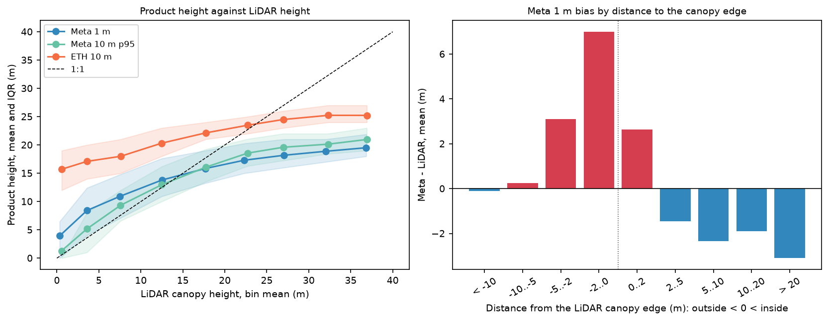
Step 7: height-class maps
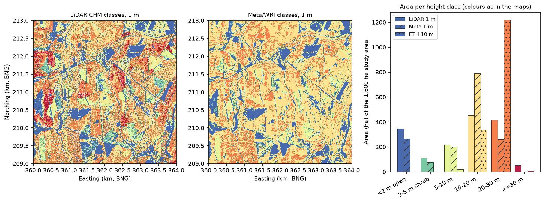
For many uses, such as habitat mapping, woodland structure or a first look at stand age, a few height classes are more honest than metres. We classify every product into the same six classes and compare areas:
CLASS_EDGES = [0, 2, 5, 10, 20, 30, 99]CLASS_NAMES = ["<2 m open", "2-5 m shrub", "5-10 m", "10-20 m", "20-30 m", ">=30 m"]

def classify(a):    c = np.digitize(a, CLASS_EDGES[1:-1]).astype("uint8")    c[np.isnan(a)] = 255    return c

cls_lid, cls_meta, cls_eth = classify(chm), classify(meta), classify(eth)write_tif(OUT / "meta_height_classes_1m_bng.tif", cls_meta, grid_tf, BNG, 255)area (ha) per height class:product LiDAR 1 m Meta 1 m ETH 10 mclass<2 m open 348.0 267.9 3.42-5 m shrub 110.4 78.5 2.05-10 m 219.5 200.9 19.310-20 m 453.5 790.8 339.320-30 m 416.3 261.4 1219.2>=30 m 52.3 0.5 6.8same class as LiDAR: Meta 1 m 46.1% of pixels; 10 m p95 classes: Meta 47.5%, ETH 49.1%Meta 1 m class within one class of LiDAR: 84.4%Meta gets the open ground, shrub and young-forest classes roughly right: 268 ha open against 348 ha in the LiDAR, and 201 ha against 220 ha at 5–10 m. Its saturation moves area out of the tall classes and into 10–20 m, which it maps at 791 ha against 454 ha. It finds almost none of the 52 ha of trees taller than 30 m. ETH’s classes are dominated by 20–30 m (1,219 ha against 416 ha) and it maps only 3.4 ha of open ground in a forest where the LiDAR finds 348 ha. Only about half of the pixels land in exactly the same class as the LiDAR for any product, but for Meta 84.4% are within one class.
Limitations and honest caveats
- Different epochs. The Meta map here is from imagery of 14 May 2018, ETH is for 2020, and the Environment Agency composite mixes surveys from November 2016 to May 2022. We could not find the survey date for this exact area. The Forest of Dean is a working forest, so stands felled or thinned between those dates count as errors. Some of ETH’s “too tall” compartments may have been felled after 2020, and some of Meta’s “too low” stands may have grown. In a forest that is harvested every year, a few per cent of the area changes between epochs.
- Leaf-off reference. The LiDAR was flown in winter. Even after pit filling, broadleaf crowns are a little lower and patchier than they would be in summer, when the satellite imagery was taken. The choice of pit filling changes Meta’s apparent bias from +1.12 m to −0.61 m, which is larger than many of the effects people try to measure.
- Saturation is the biggest error. Both maps underestimate tall forest by 7–17 m above 25 m, and neither predicts above 37 m. Do not use them for the volume or carbon of mature conifer stands without local calibration.
- Edge effects and shifts. Meta widens canopy into gaps by a few metres and is offset by about 5 m. Small gaps, narrow rides and hedgerows are the hardest features for it, and pixel-level accuracy near any edge is poor.
- Whole-metre heights. Both products store heights as integers, so they cannot resolve changes smaller than a metre and show stripes in scatter plots.
- One site. This is one 16 km² block of mixed, managed temperate forest. Accuracy will differ in open woodland, in tropical forest or on steep slopes. The Meta paper reports a mean absolute error of 2.8 m against held-out US aerial LiDAR, which is much better than we find here; a mismatch of epochs, a leaf-off reference and a forest unlike the training data all play a part.
- What counts as canopy. We use 2 m as the threshold between open ground and canopy. A different threshold changes the canopy share, the class areas and the edge distances.
Frequently asked questions
How do I download the Meta canopy height map?
You don’t need to download whole tiles. The data is public at https://dataforgood-fb-data.s3.amazonaws.com/forests/v1/alsgedi_global_v6_float/. Read tiles.geojson to find the QuadKey of the tile you need, then open chm/<quadkey>.tif with rasterio.open("/vsicurl/" + url) and read a window. For a large area, copy whole tiles with aws s3 cp s3://dataforgood-fb-data/forests/v1/alsgedi_global_v6_float/chm/<quadkey>.tif . --no-sign-request. The same data is also available in Google Earth Engine through the community catalogue.
How accurate is the Meta canopy height map?
In this test, at 1 m it has a bias of −0.61 m and an RMSE of 7.24 m against an Environment Agency LiDAR canopy height model. At 10 m the RMSE of mean height is 5.57 m. It is accurate for open ground and young stands but underestimates trees taller than about 20 m, by 9 m at 25–30 m. Treat it as a good map of where canopy is and a rough guide to height.
Is the Meta or ETH canopy height map better?
For a British forest, Meta’s map is more useful: it shows individual stands, rides and gaps at 1 m and has a smaller bias. ETH’s 10 m map has a similar correlation for tall forest but puts 15 m of canopy on open ground and compresses everything into 15–25 m. ETH has the advantage of a single, documented epoch (2020) and is easier to use for a whole country.
How do I make a canopy height model from LiDAR in Python?
Subtract a digital terrain model from a first-return digital surface model on the same grid: chm = dsm - dtm. In England both are free from the Environment Agency at 1 m. Set small negative values to zero, remove spikes, and fill pits with scipy.ndimage.grey_closing. To start from the point cloud instead, see the laspy tutorial.
Why are the canopy heights in the Meta map in Web Mercator?
The map was made in web map tiles, which use Web Mercator (EPSG:3857). That projection preserves shape locally but stretches distances by 1/cos(latitude). Reproject to a local projected CRS, such as the British National Grid (EPSG:27700), before you measure areas, compare with other data or resample to coarser cells.
Can I use these maps to estimate forest carbon?
Not on their own. Biomass and carbon depend strongly on the height of the tallest trees, which is exactly where both maps saturate. Calibrate them with local LiDAR or field plots first, and report the uncertainty.
Next steps
- Build your own canopy height model from the raw point cloud in LiDAR point clouds in Python with laspy.
- Use the same Environment Agency DSM and DTM to extract building footprints and heights from LiDAR.
- Add slope, aspect and hillshade to explain where the tallest trees grow with raster terrain analysis with rasterio.
- Track where forest has been cleared over time with deforestation detection with Global Forest Change data.
- Separate conifer from broadleaf stands with a random forest land cover classification.
Data and licences
- High Resolution Canopy Height Maps by Meta and the World Resources Institute: Tolan, J., Yang, H.-I., Nosarzewski, B., Couairon, G., Vo, H. V., Brandt, J., Spore, J., Majumdar, S., Haziza, D., Vamaraju, J., Moutakanni, T., Bojanowski, P., Johns, T., White, B., Tiecke, T. and Couprie, C. (2024), “Very high resolution canopy height maps from RGB imagery using self-supervised vision transformer and convolutional decoder trained on aerial lidar”, Remote Sensing of Environment 300: 113888. Licensed under CC BY 4.0. Read from the Registry of Open Data on AWS on 21 October 2026.
- ETH Global Canopy Height 2020: Lang, N., Jetz, W., Schindler, K. and Wegner, J. D. (2023), “A high-resolution canopy height model of the Earth”, Nature Ecology & Evolution 7: 1778–1789. Licensed under CC BY 4.0. Read from the ETH Zurich libdrive file share on 21 October 2026.
- Environment Agency LIDAR Composite DTM and First Return DSM 1 m (2022): © Environment Agency copyright and/or database right 2022. All rights reserved. Licensed under the Open Government Licence v3.0. Read through the Environment Agency Web Coverage Services on 21 October 2026.
- Natural Earth 1:50m countries: public domain.
- Code:
canopy_height.py, tested with Python 3.12.0, rasterio 1.5.2 (GDAL 3.12.2), numpy 2.5.4, scipy 1.18.1, pandas 3.0.6, shapely 2.2.0, requests 2.34.2 and matplotlib 3.11.2.
Key terms
- Canopy height model (CHM)
- A raster of vegetation height above the ground. From LiDAR it is the digital surface model minus the digital terrain model.
- DSM and DTM
- A digital surface model is the top surface, including tree crowns and roofs. A digital terrain model is the bare ground with everything above it removed.
- First-return DSM
- A surface built from the first echo of each laser pulse, which is usually the top of the canopy. The Environment Agency publishes it as the 'first return' (FZ) DSM.
- QuadKey
- A string that names a Web Mercator map tile: one digit per zoom level, each digit 0–3 choosing a quarter of the parent tile. The Meta map uses zoom-9 QuadKeys, such as 031313102.
- p95 height
- The 95th percentile of the heights inside a cell. It approximates the top of the canopy and is what most coarse canopy height products try to predict.
- Saturation
- When a model stops increasing its prediction as the true value rises, so tall canopy is systematically underestimated.
- Pit filling
- Filling small, false holes in a LiDAR CHM where pulses slipped between branches. Here a 3 × 3 greyscale closing does it.
Data for this tutorial
- Registry of Open Data on AWS · Hosts the Meta/WRI High Resolution Canopy Height Maps (s3://dataforgood-fb-data/forests/v1/)
- Global Forest Watch · Forest loss, tree cover and other forest layers to set canopy height in context
- Natural Earth · Country outlines for the tile index map
Licences and formats for each source are listed in the GIS data sources catalogue.