AlphaEarth satellite embeddings in Python: few-shot habitat mapping, uncertainty and area estimates
Use Google DeepMind's AlphaEarth Foundations satellite embeddings, a geospatial foundation model, in Python without a login. Classify nine Peak District habitats with a linear model, compare a few-shot learning curve against raw Sentinel-2 bands, map uncertainty, check calibration, simulate active learning, and estimate habitat areas with confidence intervals from a stratified random sample (Olofsson et al. 2014).
- Level
- Advanced
- Tested with
- Python 3.12
- Source code
- Download scripts
Key takeaways
- AlphaEarth Foundations 2023 embeddings with plain logistic regression reach 87.3% overall accuracy on the series' held-out spatial blocks (block-bootstrap 95% CI 84.1% to 90.2%), against 78.9% for raw seasonal Sentinel-2 bands and 60.0% for the Part 1 spectral rules.
- Few-shot: with 25 labels per class (225 in total), the embeddings score 81.2%, already better than raw Sentinel-2 bands trained on all 6,544 labels (78.9%). With 5 labels per class they score 72.0%.
- Uncertainty is informative: the least certain fifth of test samples has a 40% error rate, the most certain fifth 0.2%. Simulated uncertainty sampling reaches the accuracy of 378 random labels with 270.
- On a stratified random sample of the map, area-adjusted accuracy is 69.8% ± 1.9%, not 87%. Blanket bog covers an estimated 8,663 ± 623 ha of the 56,053 ha study area, against 8,859 ha by pixel counting.
Before you start
- Part 1 of this series, or comfort with confusion matrices, user's and producer's accuracy and spatial train/test splits
- Python 3.12 with rasterio, scikit-learn, LightGBM, pandas and matplotlib (see requirements.txt); familiarity with scikit-learn pipelines
- About 3 GB of free disk space and an internet connection; no GPU, account or API key needed
Short answer: to use AlphaEarth satellite embeddings in Python without Google Earth Engine, read the public Cloud-Optimised GeoTIFFs on Source Cooperative (tge-labs/aef) with rasterio. Each 10 m pixel has a 64-number vector per year. Turn the int8 values back into floats, sample them at your labelled points and fit a simple classifier such as logistic regression. In the Peak District this gives 87% overall accuracy for nine habitats on held-out spatial blocks, and 81% with only 25 labels per class, better than raw Sentinel-2 bands with every label. Then report the map honestly: its accuracy and class areas from a stratified random sample of the map, with confidence intervals.
Geospatial foundation models promise to do for satellite imagery what large language models did for text: learn general-purpose features once, from vast amounts of unlabelled data, so that each new mapping task needs only a handful of labels. Most tutorials stop at “here is how to extract embeddings”. This one asks the questions a habitat mapper has to answer before trusting them. How many labels do the embeddings actually save? Does the model know when it is wrong? Can it choose which places to label next? And what are the areas of each habitat, with error bars, that a peatland policy officer could quote?
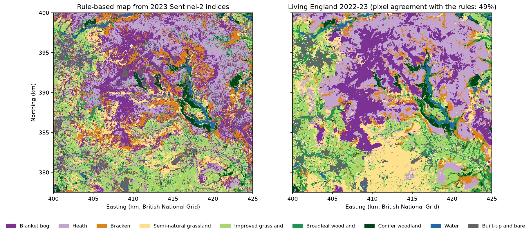
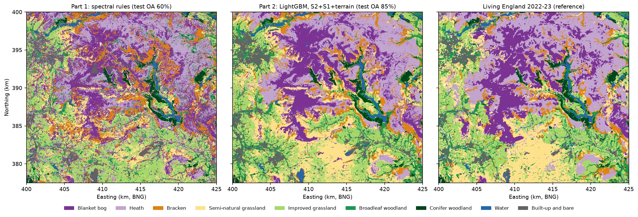
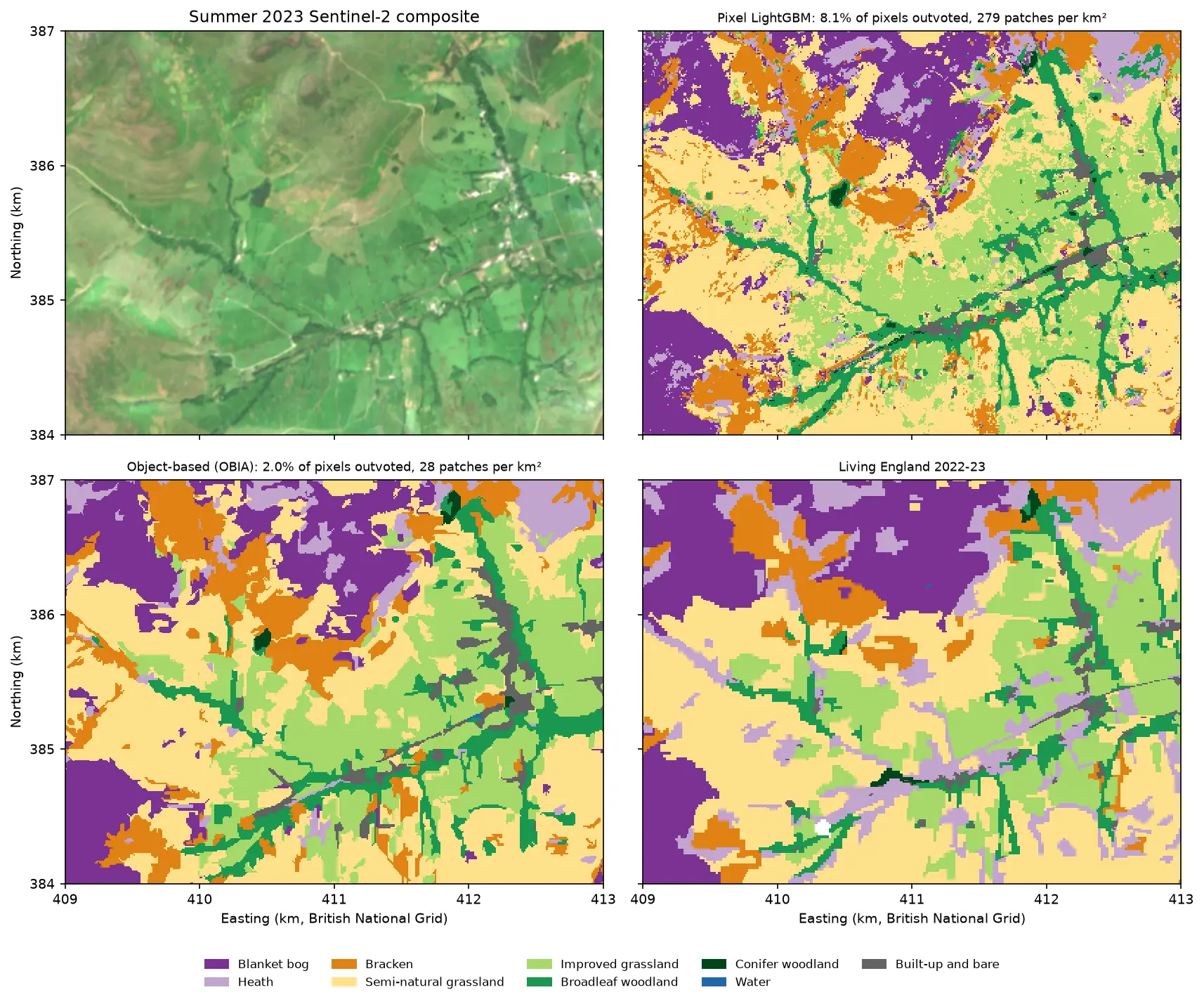
This is part 5, the last part, of AI habitat classification with Python. Every part maps the same nine habitats in the Dark Peak with the same Living England labels and the same spatial train/test split, so the numbers are directly comparable. Part 1 built the baseline with spectral index rules (60.0% overall accuracy). Part 2 used LightGBM on Sentinel-2 and Sentinel-1 features, Part 3 classified image objects (OBIA), and Part 4 trained a temporal deep learning model in PyTorch. Here the features come from a foundation model, and the classifier is deliberately simple.
You will learn how to:
- read AlphaEarth Foundations embeddings from a public bucket and put them on your own grid;
- classify habitats with a linear model on embeddings, and compare it with raw Sentinel-2 bands and other classifiers;
- draw a few-shot learning curve, the key test of a foundation model;
- map uncertainty and check calibration with a reliability diagram;
- simulate active learning with uncertainty sampling;
- estimate area-adjusted accuracy and habitat areas with 95% confidence intervals from a stratified random sample, following Olofsson et al. (2014).
All outputs below come from alphaearth_embeddings.py, its small reader module aef.py, and the series’ shared module and sample design (habitat_common.py, prepare_data.py and the sample CSVs). They were run on 21 October 2026 with Python 3.12, scikit-learn 1.9.1, LightGBM 4.7.0, rasterio 1.5.2 and pandas 3.0.6, on a laptop CPU.
What you need from earlier parts
Nothing except the shared data. You do not need to have run Parts 1 to 4. The series’ shared module and its prepare_data.py script rebuild everything in one command: the Living England labels on the 10 m grid, the committed 9,000 samples with their spatial split, and the 2023 seasonal Sentinel-2 composites that this part uses as the comparison.
py -3.12 -m venv .venv-habitat.venv-habitat\Scripts\pip install -r tutorial-code\alphaearth-satellite-embeddings-python\requirements.txt.venv-habitat\Scripts\python tutorial-code\ai-habitat-classification-common\prepare_data.py --composites.venv-habitat\Scripts\python tutorial-code\alphaearth-satellite-embeddings-python\alphaearth_embeddings.pyThe first run took 646 seconds (about 11 minutes): 583 seconds to read the embeddings over the study area (360 MB as int8), and under a minute for everything else. Later runs use the cached cube and take about 70 seconds.
The samples are the series’ design: 1,000 “pure” pixels per class from High or Very High reliability Living England polygons, in 90 blocks of 2.5 km, with 27 blocks (2,456 samples) held out for testing. All accuracies on test samples below use those 2,456 samples and nothing else. Hyperparameters are tuned only by blocked cross-validation inside the 63 training blocks.
Why AlphaEarth, and not Clay, Prithvi or SSL4EO?
Several open geospatial foundation models could provide embeddings. We picked the one that is cheapest to use correctly on a CPU:
| Option | What you get | Cost to use here |
|---|---|---|
| AlphaEarth Foundations (Google DeepMind) | Precomputed 64-d annual embeddings for every 10 m land pixel, 2017 onwards, CC BY 4.0 | Read a COG window. No GPU, no model weights |
| Clay v1.5 | Open ViT weights; embeddings per image chip | Run a ViT over the area for each date, ideally on a GPU; patch-level, not pixel-level |
| Prithvi-EO-2.0 (NASA/IBM) | Open ViT weights for HLS time series | As above; expects HLS bands and a time series |
| SSL4EO-S12 via TorchGeo | Pretrained ResNet/ViT for Sentinel-2 | Runs on CPU, but on chips; single date; per-patch features |
AlphaEarth is not just a Sentinel-2 model. It was trained on Sentinel-2, Sentinel-1, Landsat, GEDI lidar, elevation, climate and other sources, and summarises a whole year into each vector. Google publishes it in Earth Engine, which needs an account. A copy on Source Cooperative (tge-labs/aef) publishes it as public COGs with a Parquet index, so anyone can read it with rasterio. That copy is not officially supported by Google. For 2023 the study area falls in two COGs in UTM zone 30N.
That multi-sensor, full-year design matters for interpreting the results. When the embeddings beat raw Sentinel-2 bands below, the comparison is “a pretrained, multi-sensor annual summary versus four seasonal Sentinel-2 composites”, not “pretraining alone”. It is the comparison a practitioner faces, though: precomputed embeddings versus the features you would build yourself.
Step 1: read the embeddings onto the British National Grid
The mirror’s index lists every COG with its year, UTM zone and footprint. aef.find_tiles downloads it once (78 MB) and keeps the 2023 tiles that overlap the study area:
BASE = "https://data.source.coop/tge-labs/aef/v1/annual"
def find_tiles(bbox_wgs84, year, cache_dir):    """Rows of the AEF index (one per COG) that intersect a lon/lat box for one year."""    f = Path(cache_dir) / "aef_index.parquet"     # downloaded once from f"{BASE}/aef_index.parquet"    ...    df = pq.read_table(f, columns=cols, filters=[("year", "=", year)]).to_pandas()    w, s, e, n = bbox_wgs84    hit = (df.wgs84_west < e) & (df.wgs84_east > w) & (df.wgs84_south < n) & (df.wgs84_north > s)
Two details trip people up. The COGs are stored bottom-up: the geotransform has a positive pixel height, with the origin at the south-west corner. And the values are quantised to int8, with −128 as no data. aef.load_embeddings reads only the window over the study area, flips it to the usual north-up order, and reprojects it from UTM onto the series’ 10 m British National Grid with nearest-neighbour resampling. Nearest-neighbour keeps each output pixel a genuine embedding vector rather than an average of several. dequantise undoes the quantisation:
def dequantise(raw): """int8 -> float32 in [-1, 1]: (v / 127.5)^2 * sign(v); -128 (no data) -> NaN.""" v = raw.astype(np.float32) out = (v / 127.5) ** 2 * np.sign(v) out[raw == NODATA] = np.nan return outtiles = aef.find_tiles(hc.aoi_bbox_wgs84(), hc.YEAR, DATA)if not AEF_TIF.exists(): raw = aef.load_embeddings(tiles, hc.shape(), hc.transform(), hc.CRS) hc.write_geotiff(AEF_TIF, raw, nodata=aef.NODATA, dtype="int8")with rasterio.open(AEF_TIF) as src: raw = src.read() # int8 (64, 2250, 2500)samples = hc.load_samples()XE = aef.dequantise(hc.sample_values(raw, samples)) # (9000, 64) float32 in [-1, 1]2 COGs cover the study area: file zone utm_west utm_eastxrvyvkcvf8p1xhlse-0000000000-0000000000.tiff 30N 500000.0 581920.0xrvyvkcvf8p1xhlse-0000000000-0000008192.tiff 30N 581920.0 663840.0read the study-area windows and reprojected to EPSG:27700 in 583 sembedding cube (64, 2250, 2500) int8, 360 MB; valid pixels 100.00%sample embeddings (9000, 64); vector length min 0.991, median 1.000, max 1.007 (unit vectors up to 8-bit quantisation)Sentinel-2 seasonal features (9000, 40); missing values (no clear view) 0.88%The vectors have unit length, as documented, which is a useful check that the dequantisation is right. For the comparison, the same 9,000 samples are also described by the ten Sentinel-2 bands of each of the four 2023 seasonal composites from the shared module: 40 raw features.
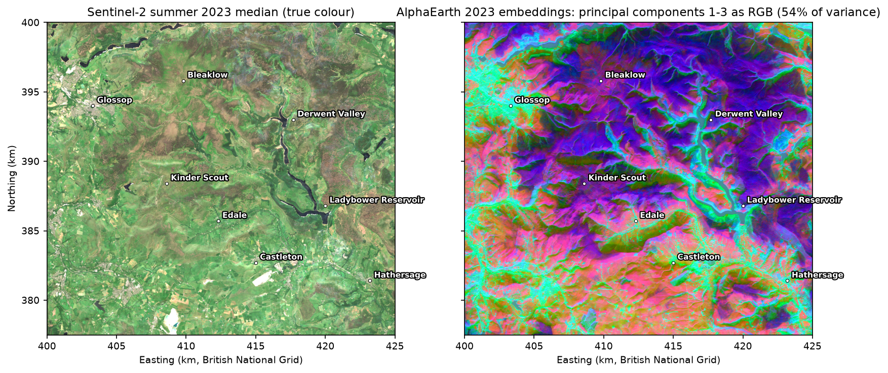
Embeddings have no physical units, but you can look at them. Projecting the 64 dimensions onto their first three principal components and showing those as red, green and blue gives a false-colour image of what the model “sees”:
Step 2: a linear classifier on the embeddings
Foundation-model embeddings are meant to make the classifier’s job easy, so we start with the simplest sensible one: logistic regression after standardising each feature. The regularisation strength C is chosen by blocked 5-fold cross-validation inside the training blocks, separately for each feature set:
def logreg(C=1.0):    return make_pipeline(SimpleImputer(strategy="median"), StandardScaler(), LogisticRegression(C=C, max_iter=3000))
for fname, X in FEATS.items(): # AlphaEarth (64) and Sentinel-2 seasonal bands (40) for C in (0.01, 0.1, 1.0, 10.0): accs = [] for k in range(5): # the series' spatial folds, training blocks only trk, vak = is_tr & (fold != k), is_tr & (fold == k) accs.append((logreg(C).fit(X[trk], y[trk]).predict(X[vak]) == y[vak]).mean())features AlphaEarth embeddings (64) Sentinel-2 seasonal bands (40)C0.01 0.874 0.7920.10 0.880 0.8161.00 0.880 0.82910.00 0.874 0.826chosen C: AlphaEarth embeddings (64): 0.1; Sentinel-2 seasonal bands (40): 1Then each feature set is fitted on all 6,544 training samples with three classifiers, and scored on the 2,456 test samples:
features AlphaEarth embeddings (64) Sentinel-2 seasonal bands (40)classifierLightGBM (300 trees) 0.860 0.792k-nearest neighbours (k=10) 0.819 0.738logistic regression 0.873 0.789Two things stand out. The embeddings beat the raw bands by 7 to 8 points with every classifier. And on the embeddings, a linear model beats LightGBM. On raw bands the non-linear LightGBM is the better choice, because it has to learn how bands combine. The embeddings have already done that work, so a gradient-boosted model has little left to add and more room to overfit. That is the practical meaning of “linearly separable features”.
The confusion matrix of the logistic regression on embeddings:
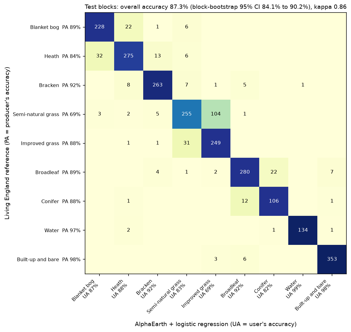
n_test producers_acc users_acc f1Blanket bog 257 0.887 0.867 0.877Heath 326 0.844 0.884 0.863Bracken 285 0.923 0.916 0.920Semi-natural grassland 370 0.689 0.833 0.754Improved grassland 282 0.883 0.694 0.777Broadleaf woodland 316 0.886 0.921 0.903Conifer woodland 120 0.883 0.822 0.851Water 138 0.971 0.993 0.982Built-up and bare 362 0.975 0.975 0.975overall accuracy 0.873 (n = 2,456); block-bootstrap 95% CI 0.841 to 0.902macro F1 0.878; Cohen's kappa 0.855; Part 1 rules: OA 0.600The two classes that defeated Part 1 have improved the most. Blanket bog’s user’s accuracy rises from 0.41 to 0.87, so bog is no longer over-mapped onto heath. Semi-natural grassland’s producer’s accuracy rises from 0.23 to 0.69. It is still the weakest class, and most of its errors (104 of 115) are still “improved grassland”. That boundary is partly a matter of management and history that no satellite sees clearly, and Living England itself is least sure there.
Predicting all 5.6 million pixels takes 8 seconds. The block loop also keeps the top probability, the margin between the two most likely classes, and the normalised entropy for every pixel, which Step 4 uses:
predicted 5,625,000 pixels in 8 swall-to-wall agreement with Living England: whole area 0.693; test blocks 0.700; training blocks 0.689 (Part 1 rules: 0.490 and 0.483)mean entropy 0.258; pixels with margin < 0.2: 14.9%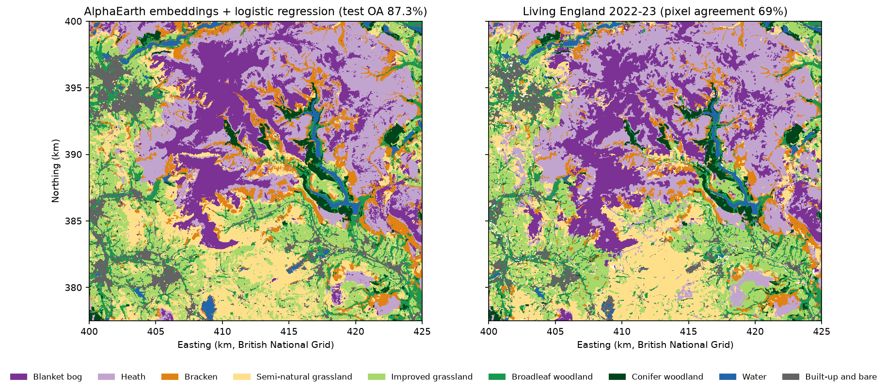
Agreement with Living England over every pixel (69%) is far below the test-sample accuracy (87%). The test samples are pure pixels in the cores of reliable polygons, while the map also covers edges, mixtures and Living England’s own less reliable polygons. Agreement is the same in test blocks (0.700) and training blocks (0.689), so the model is not memorising the training areas. Step 6 turns this gap into a proper estimate.
Step 3: the few-shot learning curve
The reason to use a foundation model is to need fewer labels. To measure that, we draw n training samples per class at random from the training blocks, fit the classifier, score it on the full test set, and repeat 20 times for each n. To keep the comparison fair, both feature sets use fixed settings here (logistic regression with C = 1, and kNN with k = 5), because tuning on five samples per class is not meaningful.
SHOTS = [5, 10, 25, 50, 100, 250]tr_idx_by_class = {c: np.flatnonzero(is_tr & (y == c)) for c in IDS}for fname, X in FEATS.items(): for n in SHOTS + ["all"]: for rep in range(REPEATS if n != "all" else 1): g = np.random.default_rng(10_000 + rep) if n == "all": sel = np.flatnonzero(is_tr) else: sel = np.concatenate([g.choice(tr_idx_by_class[c], n, replace=False) for c in IDS]) m = logreg(1.0).fit(X[sel], y[sel]) # and the same with k-nearest neighbours acc = (m.predict(X[is_te]) == y[is_te]).mean() AlphaEarth embeddings (64) Sentinel-2 seasonal bands (40)per_class5 0.720 0.63010 0.767 0.67225 0.812 0.72150 0.829 0.743100 0.850 0.767250 0.867 0.781all 0.875 0.789AlphaEarth + logistic regression with 25 labels per class (0.812) already matches Sentinel-2 bands with all 6,544 training labels (0.789)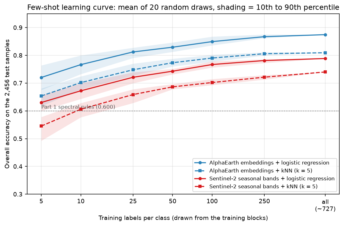
This is the central result. With 25 labels per class, 225 in total, the embeddings beat raw Sentinel-2 bands trained on all 6,544 labels. With 5 per class, 45 labels that one person could check on aerial photographs in an afternoon, they reach 72%, comfortably above the hand-tuned rules of Part 1. The gap is largest when labels are scarce (9 points at 5 per class) and narrows but never closes. The kNN curves tell the same story at a lower level: the embedding space is well organised enough that “label of the most similar pixels” works too.
Step 4: uncertainty and calibration
A logistic regression gives a probability for every class. Two summaries are useful for mapping. The margin is the top probability minus the runner-up, where small means “torn between two habitats”. The entropy is spread over all nine classes. Both are computed for every pixel in Step 2’s prediction loop. If the uncertainty means anything, errors should cluster where the margin is small:
margin_from margin_to error_rate nlowest 0.001 0.439 0.400 492low 0.439 0.782 0.171 491middle 0.783 0.943 0.041 491high 0.943 0.994 0.022 491highest 0.994 1.000 0.002 491expected calibration error on the pure test samples: 0.022The least certain fifth of the test samples has 40% errors, the most certain fifth 0.2%. The uncertainty is clearly informative. Calibration asks a stricter question: when the model says 0.8, is it right 80% of the time? A reliability diagram bins the predictions by their top probability and plots the observed accuracy in each bin. The expected calibration error (ECE) is the weighted mean gap between the two.
On the pure test samples the model is well calibrated (ECE 0.022). But those samples are not what the map is made of. The same check on the stratified random sample of the map from Step 6, weighted by the area each sample point represents, tells a different story:
conf_map = pmax.ravel()[pts] # top probability at each map-sample pixelw_map = (mapped / n_h)[np.searchsorted(IDS, s_map)] # each sampled pixel stands for this many map pixelsrel_map, ece_map = reliability(conf_map, s_map == s_ref, w=w_map)expected calibration error on the stratified map sample (area-weighted): 0.088 (pure test samples: 0.022)area-weighted mean confidence on the map 0.783 vs area-adjusted overall accuracy 0.698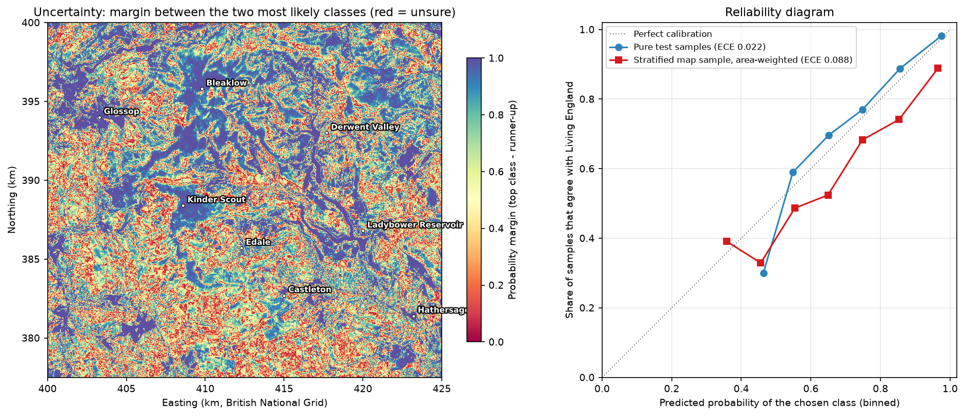
Across the whole map the model is overconfident: its mean confidence is 0.78, but it agrees with Living England only 70% of the time. Calibration measured on clean, balanced test points does not carry over to mixed pixels, field edges and the places where the reference itself is shaky. Use the uncertainty map to rank places for checking, which it does well, rather than reading its probabilities as literal chances of being right.
Step 5: active learning with uncertainty sampling
If the model knows where it is unsure, it can choose what to label next. We simulate that. The 6,544 training samples are the unlabelled “pool”, and their labels are revealed only when the strategy picks them. We start with 2 labels per class, then add batches of 18 for 20 rounds. Uncertainty sampling picks the 18 pool samples with the smallest margin; random sampling picks 18 at random. Each strategy is run 10 times from the same starting sets, and every model is scored on the untouched test blocks.
for rnd in range(ROUNDS + 1): m = LogisticRegression(C=1.0, max_iter=3000).fit(Zp[lab], yp_pool[lab]) ... rest = np.setdiff1d(np.arange(len(pool)), lab) if strategy == "random": new = g.choice(rest, BATCH, replace=False) else: P = np.sort(m.predict_proba(Zp[rest]), 1) new = rest[np.argsort(P[:, -1] - P[:, -2])[:BATCH]] # smallest margin first lab.extend(new.tolist()) mean stdstrategy random uncertainty random uncertaintyn_labels18 0.645 0.645 0.050 0.05090 0.746 0.783 0.020 0.023162 0.779 0.811 0.024 0.018234 0.803 0.819 0.025 0.018306 0.816 0.826 0.023 0.021378 0.821 0.838 0.026 0.023random sampling reaches 0.821 with 378 labels; uncertainty sampling reaches it with 270 labels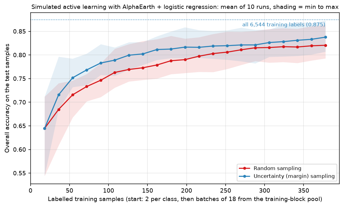
Uncertainty sampling reaches the accuracy of 378 random labels with 270, saving about 30% of the labelling effort, and its lead is largest early on (78.3% against 74.6% at 90 labels). The runs overlap, so in any one project the gain could be smaller. The simulation is also kind to active learning: the pool contains only pure, balanced samples, so the “most uncertain” pixel is always a genuine, labellable example of one class. In a real map, the most uncertain pixels are often mixed pixels and field edges that a person cannot label confidently either. Filter them out, or sample uncertain patches, before sending them to an interpreter.
Step 6: area-adjusted accuracy and habitat areas
Everything so far measured accuracy on the series’ test samples: balanced, 1,000 per class before the split, from pure pixels in reliable polygons. That is a fair way to compare methods, which is what this series needs. It is not an estimate of how accurate the map is, or of how much of each habitat there is. Bog is not 1/9 of the area, and the map’s errors concentrate exactly where the samples were not allowed to go.
Good practice, set out by Olofsson et al. (2014), is to assess a map with a probability sample of the map itself. The usual design is a stratified random sample with the mapped classes as strata. Each sampled pixel gets a reference label, and stratified estimators then give overall accuracy, user’s and producer’s accuracy and the area of each class, with standard errors. The series’ test samples were not drawn that way: their inclusion probabilities are unknown and unrelated to the map. So we draw a proper sample.
popn = (labels > 0) & (pred > 0) # Living England labels every pixel except fen and the edgesmapped = np.array([(pred[popn] == c).sum() for c in IDS], float)W = mapped / mapped.sum()N_TOTAL, N_MIN = 2000, 100n_h = np.maximum(N_MIN, np.round(W * N_TOTAL)).astype(int)g = np.random.default_rng(hc.SEED)flat_pred = np.where(popn, pred, 0).ravel()pts = []for c, n in zip(IDS, n_h): pts.append(g.choice(np.flatnonzero(flat_pred == c), n, replace=False))pts = np.concatenate(pts)s_map = flat_pred[pts]s_ref = labels.ravel()[pts] # reference: Living England at each sampled pixelThe sample allocates about 2,000 pixels in proportion to mapped area, with at least 100 per class so that rare classes such as water get usable estimates, and a fixed seed. The reference label at each pixel is Living England, with no reliability or purity filter: the map is judged against Living England everywhere, edges included. The estimators are the stratified ones of Olofsson et al. (2014):
def olofsson(map_cls, ref_cls, mapped_px, px_ha=0.01): """Stratified estimators of Olofsson et al. (2014): strata = map classes, weights = mapped area shares.""" nij = pd.crosstab(pd.Categorical(map_cls, IDS), pd.Categorical(ref_cls, IDS), dropna=False).to_numpy().astype(float) ni = nij.sum(1) W = mapped_px / mapped_px.sum() p = W[:, None] * nij / ni[:, None] # estimated area proportions (map i, reference j) pj = p.sum(0) ua = np.diag(nij) / ni se_oa = np.sqrt((W ** 2 * ua * (1 - ua) / (ni - 1)).sum()) se_pj = np.sqrt((W[:, None] ** 2 * (nij / ni[:, None]) * (1 - nij / ni[:, None]) / (ni[:, None] - 1)).sum(0)) ... # producer's accuracy and its standard error A = mapped_px.sum() * px_ha return {"oa": np.trace(p), "se_oa": se_oa, "area_ha": pj * A, "se_area_ha": se_pj * A, ...}population 5,605,307 pixels (56,053 ha); stratified sample n = 2,107 (at least 100 per mapped class, the rest proportional to mapped area; seed 42)reference = Living England 2022-23 at each sampled pixel, any reliability, no purity filterareas (ha) and the Living England census of the same population: n_sample mapped_ha adjusted_ha ci95_ha le_ha le_in_ciBlanket bog 316 8859 8663 623 9052 TrueHeath 433 12130 14691 718 15145 TrueBracken 195 5475 4277 499 4156 TrueSemi-natural grassland 340 9542 9427 779 9610 TrueImproved grassland 345 9663 9688 731 8996 TrueBroadleaf woodland 149 4182 4085 462 3967 TrueConifer woodland 100 1543 1702 242 1719 TrueWater 100 1036 966 159 839 TrueBuilt-up and bare 129 3622 2554 341 2570 Truearea-adjusted user's and producer's accuracy with 95% CI half-widths: users_acc ua_ci95 prod_acc pa_ci95Blanket bog 0.744 0.048 0.760 0.041Heath 0.873 0.031 0.721 0.031Bracken 0.595 0.069 0.762 0.062Semi-natural grassland 0.553 0.053 0.560 0.042Improved grassland 0.652 0.050 0.650 0.041Broadleaf woodland 0.671 0.076 0.687 0.062Conifer woodland 0.810 0.077 0.734 0.093Water 0.770 0.083 0.826 0.116Built-up and bare 0.628 0.084 0.891 0.056area-adjusted overall accuracy 0.698 +/- 0.019 (95% CI); compare 0.873 on the balanced, pure test samplessample points in test blocks: 616 (agreement 0.714); in training blocks: 1491 (agreement 0.698)blanket bog: mapped 8,859 ha; adjusted 8,663 ha (95% CI 8,041 to 9,286); Living England census 9,052 haLiving England census inside the 95% CI for 9 of 9 classes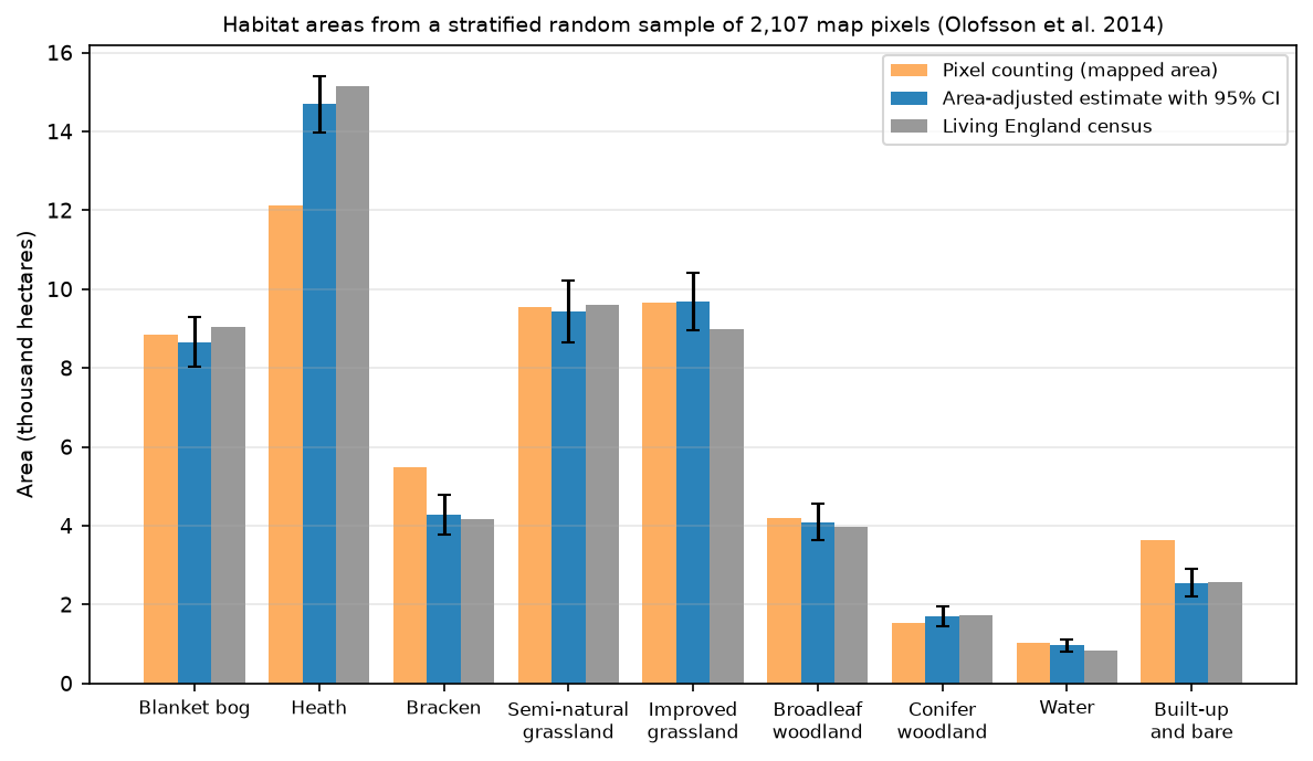
Area-adjusted overall accuracy is 69.8% ± 1.9%, not 87%. That is the accuracy of the map, judged against Living England, over the whole study area. Per class, user’s accuracy for blanket bog is 0.74 ± 0.05 and producer’s accuracy 0.76 ± 0.04. The map over-maps bracken (mapped 5,475 ha, estimated 4,277 ± 499 ha) and built-up and bare land (3,622 against 2,554 ± 341 ha), and under-maps heath (12,130 against 14,691 ± 718 ha). Pixel counting would report those biases as facts. The adjusted estimates correct them.
For blanket bog, the habitat that matters most for peatland carbon policy, the estimate is 8,663 ha (95% CI 8,041 to 9,286 ha), about 15% of the study area. Pixel counting gives 8,859 ha, inside the interval. Because the reference here is Living England, we can check the method against a census of the same population. Living England’s own bog area is 9,052 ha, inside the interval, and the census falls inside the 95% interval for all nine classes. The estimator does what it promises: about 2,000 labelled pixels recover the reference areas to within a few per cent.
Two caveats are important. First, the sample includes pixels in the training blocks, whose cores supplied training samples. Agreement at sample points in test blocks (0.714) and training blocks (0.698) is the same within sampling error, so this does not inflate the estimate. Second, the result is still “accuracy against Living England”. For a real bog inventory, the reference at each sample pixel should come from field survey or careful photo-interpretation, not from another map.
misuse check, the 2,456 pure test samples plugged into the same estimator: 'area-adjusted' OA 0.852; blanket bog 8,744 +/- 525 haFive methods compared: which should you use?
Each part of this series reports the same measures on the same 2,456 test samples in the same 27 held-out blocks, so the methods can be compared directly. For the two ends of the series:
| Measure (test blocks, n = 2,456) | Part 1: spectral rules | Part 5: AlphaEarth + logistic regression |
|---|---|---|
| Overall accuracy (block-bootstrap 95% CI) | 0.600 (0.527 to 0.664) | 0.873 (0.841 to 0.902) |
| Macro F1 | 0.630 | 0.878 |
| Cohen’s kappa | 0.547 | 0.855 |
| Semi-natural grassland, producer’s accuracy | 0.227 | 0.689 |
| Blanket bog, user’s accuracy | 0.407 | 0.867 |
| Wall-to-wall agreement with Living England, test blocks | 0.483 | 0.700 |
Parts 2 to 4 sit between these two approaches. Part 2 trains LightGBM on seasonal Sentinel-2, Sentinel-1 radar and terrain features. Part 3 segments the image into objects and classifies them (OBIA). Part 4 trains a temporal neural network in PyTorch on each pixel’s Sentinel-2 time series. Here are all five, from each part’s recorded console output and metrics.json:
| Part | Method | OA (95% CI) | Macro F1 | Kappa | Wall-to-wall, test blocks | Runtime | Notes |
|---|---|---|---|---|---|---|---|
| 1 | Eight spectral index rules, seasonal Sentinel-2 | 0.600 (0.527–0.664) | 0.630 | 0.547 | 0.483 | about 15 s | Noisy map; bog over-mapped (UA 0.41), semi-natural grassland PA 0.23 |
| 2 | LightGBM, 77 features: Sentinel-2, Sentinel-1 and terrain | 0.853 (0.801–0.892) | 0.862 | 0.833 | 0.687 | 3.0 min | Radar adds +0.011 (not significant), terrain +0.052; Sentinel-2 alone 0.790 |
| 3 | Object-based LightGBM, Felzenszwalb segments, Sentinel-2 only | 0.794 (0.729–0.845) | 0.808 | 0.766 | 0.642 | 9.5 min | Cleanest map: 17 patches/km² against 196 for pixels (Living England 17); same accuracy as pixels (0.797) |
| 4 | TempCNN on 50 raw Sentinel-2 dates + clear mask, 3-seed ensemble | 0.851 (0.811–0.884) | 0.858 | 0.830 | 0.699 | 19.2 min | LightGBM on the same dates 0.842, not a significant win; keeps 0.824 with half the clear views (LightGBM 0.535) |
| 5 | AlphaEarth embeddings + logistic regression | 0.873 (0.841–0.902) | 0.878 | 0.855 | 0.700 | 10.8 min | 0.812 with 25 labels per class; area-adjusted OA 0.698 ± 0.019; bog 8,663 ± 623 ha |
OA is overall accuracy on the same 2,456 test samples in 27 held-out blocks, with a 2,000-resample block-bootstrap 95% interval. Wall-to-wall agreement is the share of every labelled Living England pixel in the test blocks that the map matches, including edges and mixed pixels. Runtimes are on one laptop CPU after prepare_data.py --composites has cached the Sentinel-2 and Sentinel-1 composites; Part 4 includes 11.3 minutes to download a 50-date stack and map every pixel, and Part 5 includes about 10 minutes to read the embeddings for the first time.
How to read the table:
- Every method beats the rules by a wide margin. Parts 2 to 5 gain 19 to 27 points of overall accuracy on Part 1, far outside the uncertainty, and the two classes that defeated the rules (bog and semi-natural grassland) gain the most.
- Parts 2, 4 and 5 are statistically tied on accuracy. 0.853, 0.851 and 0.873 have overlapping block-bootstrap intervals, and the 2-point lead of the embeddings is smaller than the width of any of them. With 27 test blocks, this design cannot rank them, and you should not either.
- Part 3 is lower because of its inputs, not its objects. It uses Sentinel-2 seasonal features only. On those, Part 2’s pixel LightGBM scores 0.790 and Part 3’s own pixel model 0.797, so objects change the look of the map, not its accuracy.
- The real advantage of the embeddings is labels, not points. With 25 labels per class they reach 0.812, already better than raw Sentinel-2 bands with all 6,544 labels (0.789), and the classifier is a few lines of scikit-learn. Parts 2 and 4 used every training label, about 727 per class, plus feature engineering or a deep learning pipeline, to reach the same level.
- None of these numbers is map accuracy. On a stratified random sample of the whole map, this part’s accuracy is 0.698, not 0.873. Expect the same drop for the others: their wall-to-wall agreement, 0.64 to 0.70, tells the same story.
Some general lessons hold whatever the exact ranking:
- Start with rules (Part 1) when you need a transparent, explainable map, have almost no labels, or must justify every decision to a non-specialist. Expect them to fail on the confusable upland classes.
- Use gradient boosting on engineered features (Part 2) as the default workhorse when you have hundreds of labels per class and want control over the inputs. Terrain gave the biggest boost here, radar a small one, and feature importance gives some interpretability.
- Use object-based analysis (Part 3) when the map is for people who draw polygons. Field and parcel boundaries matter, and salt-and-pepper noise is unacceptable even if pixel accuracy hardly changes.
- Use temporal deep learning (Part 4) when you have many labels, dense but gappy time series and a phenology-driven question, such as when a habitat greens up or is cut. It copes far better than LightGBM when clear views are missing, but costs more effort and compute than the others.
- Use foundation-model embeddings (this part) when labels are scarce or expensive, when you want a strong map quickly, or as a baseline that any custom model must beat. Accept the costs: the features cannot be interpreted, they are fixed at one vector per year, and you depend on the provider’s choices of inputs, years and versions.
Whatever you choose, assess the final map with a stratified random sample and report areas with confidence intervals, as in Step 6. The test-sample accuracy is for choosing a method. The area-adjusted accuracy is for the people who will use the map.
Limitations
- The labels are a model. Every number here measures agreement with Living England, not with the ground. Living England is itself made from Sentinel-1 and Sentinel-2 imagery, and AlphaEarth uses both sensors as well, so the two may share some biases. That would flatter both the embeddings and the raw bands.
- Balanced, pure samples. The 87% applies to clean pixels of nine equally weighted classes. The map’s accuracy is 70% (Step 6).
- An annual summary. One vector per year cannot show when something happened, such as a burn, a cut or a flood. Use time series for that (Part 4).
- No interpretability. You cannot say why a pixel is bog. The 64 dimensions have no physical meaning, and they may change between dataset versions.
- Dependency. The embeddings are produced by Google and Google DeepMind. The Source Cooperative copy is an unofficial mirror with no guarantee of continuity. Cache what you use and record the version (here
v1, annual, 2023). - Simulations, not field campaigns. The few-shot and active-learning results use labels that already exist. Real labels cost money, have errors and are not all equally easy to collect.
Frequently asked questions
What are AlphaEarth Foundations satellite embeddings?
They are the output of Google DeepMind’s AlphaEarth Foundations model: one 64-dimensional vector for every 10 m pixel of land, for each year from 2017. The model was trained on optical, radar, lidar, elevation, climate and other data, and summarises a pixel’s whole year. Similar places get similar vectors, so a simple classifier on the vectors can map land cover, crops or habitats from few labels. The dataset is licensed CC BY 4.0.
Can I use AlphaEarth embeddings without Google Earth Engine?
Yes. A public mirror on Source Cooperative (tge-labs/aef) holds the annual embeddings as Cloud-Optimised GeoTIFFs with a Parquet index, under the same CC BY 4.0 licence. You can read a window with rasterio over HTTPS with no account, as in Step 1. Note that the files are stored bottom-up and quantised to int8, so flip the rows and dequantise the values.
How many training samples do I need with foundation-model embeddings?
Far fewer than with raw bands. In this study, 5 labels per class gave 72% accuracy and 25 per class gave 81%, already better than raw Sentinel-2 bands with all 6,544 labels. A few dozen good labels per class is a reasonable start, with more for classes that are easily confused, such as semi-natural and improved grassland.
Which classifier should I use on embeddings?
Start with a linear model such as logistic regression, with standardised features and a regularisation strength chosen by spatial cross-validation. Here it beat both k-nearest neighbours and LightGBM. Embeddings are designed to be linearly separable, so a flexible model adds little and can overfit. A linear model is also fast and gives usable probabilities for uncertainty maps and active learning.
How do I estimate the area of a land cover class with confidence intervals?
Draw a stratified random sample from your map, with the mapped classes as strata. Get a reliable reference label for each sample pixel, then apply the stratified estimators of Olofsson et al. (2014). These weight each stratum by its mapped area and give each class’s area with a standard error. Do not reuse training or convenience test samples: their inclusion probabilities are unknown, so the estimates are biased and the intervals too narrow.
Are geospatial foundation models better than training my own model?
Often, when labels are scarce. With plenty of labels and dense time series, a well-built custom model can match or beat them on a specific task, and it gives you control and interpretability. Embeddings are an excellent first baseline: quick to try and hard to beat for their cost.
Try it yourself
- Another year. Set
hc.YEARto 2022 for the embeddings only, and classify 2022 with the 2023 model. How much does accuracy drop, and which classes change? This tests whether embeddings are stable from year to year. - Change detection. Download the 2018 embeddings as well and compute the cosine similarity between 2018 and 2023 for each pixel. Map the 1% least similar pixels. Do they pick out moorland fires, felled conifer plantations or new buildings?
- Similarity search. Take the mean embedding of 20 blanket bog training pixels on Kinder Scout and map the cosine similarity of every pixel to it. Where else does the model see “Kinder-like” bog, and where does that disagree with Living England?
- A better sampling design. Re-run Step 6 with Neyman allocation, which gives larger samples to strata with lower user’s accuracy, and compare the width of the bog interval with the proportional design.
- Your own labels. Replace Living England at 200 of the stratified sample pixels with your own photo-interpretation from aerial imagery. How different is the area-adjusted accuracy when the reference is not another map?
Next steps
- Go back to the start of the series with habitat mapping with Sentinel-2 in Python, the rule-based baseline and the full explanation of the spatial split.
- Compare the other methods in depth: LightGBM with Sentinel-2, Sentinel-1 and terrain (Part 2), object-based image analysis (Part 3) and time series deep learning in PyTorch (Part 4).
- Compare a classic supervised workflow on global labels in land cover classification with a Sentinel-2 random forest.
- Turn the habitat and uncertainty rasters into statistics per moorland unit or catchment with zonal statistics in Python.
- For image-chip deep learning, see training data for deep learning on satellite imagery, train a U-Net and inference over large rasters. For another pretrained model, try Segment Anything on satellite imagery.
- Share the maps on the web with interactive web maps with Folium.
Data and licences
- AlphaEarth Foundations Satellite Embedding dataset, annual, v1, 2023: licensed CC BY 4.0. “The AlphaEarth Foundations Satellite Embedding dataset is produced by Google and Google DeepMind.” Accessed from the public Source Cooperative mirror tge-labs/aef on 21 October 2026. Brown, C. F. et al. (2025), “AlphaEarth Foundations: An embedding field model for accurate and efficient global mapping from sparse label data”, arXiv:2507.22291.
- Living England Habitat Map 2022-23: © Natural England, under the Open Government Licence v3.0. Contains Ordnance Survey data © Crown copyright and database right. Accessed from Natural England’s public ArcGIS service on 21 October 2026.
- Sentinel-2 L2A: contains modified Copernicus Sentinel data 2023, free and open under the Copernicus data licence. Accessed from the Microsoft Planetary Computer.
- Reference: Olofsson, P., Foody, G. M., Herold, M., Stehman, S. V., Woodcock, C. E. and Wulder, M. A. (2014), “Good practices for estimating area and assessing accuracy of land change”, Remote Sensing of Environment 148, 42–57.
- Code:
alphaearth_embeddings.pyandaef.pyand the shared series module (habitat_common.py,prepare_data.py, sample CSVs), tested with Python 3.12.0, scikit-learn 1.9.1, LightGBM 4.7.0, rasterio 1.5.2, numpy 2.5.4, pandas 3.0.6 and matplotlib 3.11.2.
Key terms
- Geospatial foundation model
- A large model pretrained on huge amounts of unlabelled Earth observation data, which can then be reused for many tasks with few labels, by fine-tuning it or by using its outputs (embeddings) as features.
- Embedding
- A vector of numbers that summarises a pixel or a patch, learned so that similar places get similar vectors. AlphaEarth embeddings have 64 dimensions per 10 m pixel per year.
- Few-shot learning
- Learning a task from very few labelled examples per class, typically 1 to 50. Good pretrained features are what make it possible.
- Active learning
- An iterative labelling strategy in which the model chooses which samples a person should label next, usually those it is least sure about.
- Calibration
- How well predicted probabilities match observed frequencies. A calibrated model is right about 80% of the time when it says 0.8. A reliability diagram plots one against the other.
- Area-adjusted accuracy
- Accuracy and class areas estimated from a probability sample of the map, weighting each stratum by its mapped area, as recommended by Olofsson et al. (2014). It describes the map, not a set of convenient test points.
Data for this tutorial
- AlphaEarth Satellite Embeddings · Public mirror of the AlphaEarth Foundations Satellite Embedding dataset (tge-labs/aef), no login
- Living England Habitat Map · Natural England's broad habitat map, used as labels and as the reference for the map sample
- Microsoft Planetary Computer · Sentinel-2 L2A for the raw-band comparison, no account needed
Licences and formats for each source are listed in the GIS data sources catalogue.