Habitat classification with LightGBM in Python: Sentinel-2, Sentinel-1 and terrain fusion
Classify nine upland habitats in the Peak District with LightGBM on 77 multi-temporal features: seasonal Sentinel-2 bands and indices, Sentinel-1 VV and VH backscatter and Copernicus DEM terrain. Tune with spatial-fold cross-validation and class weights, run an S2 / S2+S1 / S2+S1+terrain ablation, explain the model with TreeSHAP and permutation importance, and compare it with a random forest and the Part 1 rules on the same test blocks.
- Level
- Intermediate
- Tested with
- Python 3.12
- Source code
- Download scripts
Key takeaways
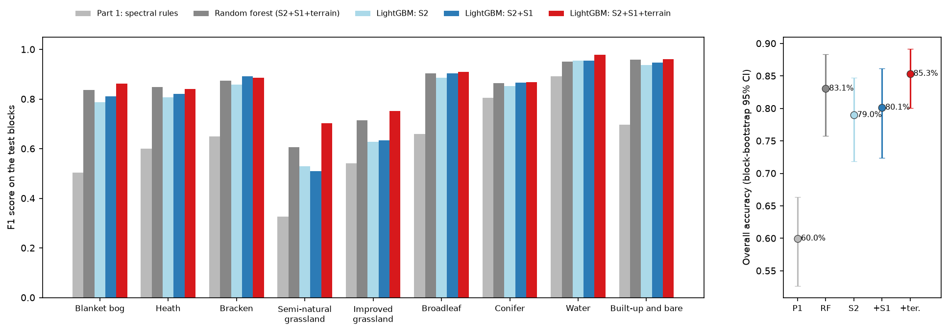
- LightGBM on 77 multi-temporal features maps nine Dark Peak habitats with 85.3% overall accuracy on the held-out test blocks (block-bootstrap 95% CI 80.1% to 89.2%), a macro F1 of 0.86 and kappa 0.83. The Part 1 spectral rules scored 60.0% on exactly the same test pixels.
- Features matter more than the algorithm. LightGBM on Sentinel-2 alone reached 79.0%; adding Sentinel-1 radar gave +1.1 points (95% CI −0.1 to +2.6) and adding elevation and slope a further +5.2 (+2.2 to +9.2).
- Sentinel-1 helped bog and heath a little (bog F1 0.79 to 0.81, confusions 73 to 69) but not semi-natural versus improved grassland. Terrain fixed the grasslands: their confusions fell from 250 to 155 and semi-natural grassland F1 rose from 0.51 to 0.70.
- A random forest on the same 77 features scored 83.1%, so LightGBM's edge is real but small (+2.3 points, CI +0.3 to +4.8). Random 5-fold cross-validation reported 89.4% for the model that scored 86.7% with spatial folds and 85.3% on the test blocks.
Before you start
- Part 1 of this series, Habitat mapping with Sentinel-2 in Python, for the study area, labels, shared split and accuracy assessment
- Python 3.12 with lightgbm, scikit-learn, odc-stac, pystac-client, planetary-computer, rasterio, pandas and matplotlib (see requirements.txt)
- About 2.5 GB of free disk space, 8 GB of RAM and an internet connection; no GPU, account or API key needed
Short answer: for LightGBM land cover or habitat classification in Python, sample a stack of per-pixel features at labelled points. Use seasonal Sentinel-2 bands and indices, seasonal Sentinel-1 VV, VH and VH/VV in decibels, and terrain from a DEM. Train lightgbm with a multiclass objective and class weights, and tune it with spatial folds of whole blocks, letting early stopping choose the number of trees. Then predict the whole raster in chunks. In the Dark Peak this reaches 85% overall accuracy across nine habitats on held-out blocks, against 60% for Part 1’s spectral rules. Terrain added more than radar did.
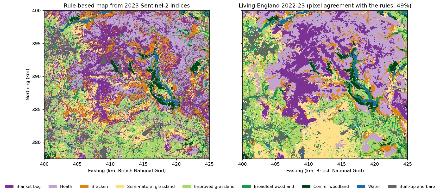
Part 1 of this series mapped blanket bog, heath, bracken, grassland, woodland, water and built-up land in the Dark Peak with eight spectral index rules, and scored 60% on held-out spatial blocks. The rules were transparent, but they could only use a handful of features and straight thresholds. This tutorial keeps everything else identical: the same 10 m grid, the same Living England labels, the same 9,000 samples and the same train/test blocks. It hands the problem to a machine-learning classifier that can use 77 features at once.
The features fuse three sensors. Sentinel-2 gives four seasonal composites of ten bands, plus indices for greenness, water, moisture and the red edge. Sentinel-1 radar gives seasonal VV and VH backscatter, which responds to structure and wetness rather than colour, and sees through cloud. The Copernicus DEM gives elevation and slope, which matter in the uplands because blanket bog forms on gentle, high, wet ground. The classifier is LightGBM, a gradient boosting library, and an ablation shows what each sensor adds. The focus is on the two hardest pairs from Part 1: bog versus heath, and semi-natural versus improved grassland.
This is part 2 of five in AI habitat classification with Python. Later parts use the same split, so their numbers compare directly with the ones here. Part 3 moves from pixels to image objects (OBIA), Part 4 trains a temporal deep learning model on each pixel’s full Sentinel-2 time series, and Part 5 tries pretrained geospatial foundation model embeddings with few-shot and active learning.
You will learn how to:
- build a multi-temporal, multi-sensor feature stack of Sentinel-2, Sentinel-1 and terrain on one grid;
- tune LightGBM with spatial-fold cross-validation, early stopping and class weights;
- run an ablation (S2, S2+S1, S2+S1+terrain) and test the differences with a paired block bootstrap;
- explain the model with gain, TreeSHAP and grouped permutation importance;
- compare it fairly with a random forest and the Part 1 rules on the identical test pixels;
- map the whole area with a confidence layer, and see how sample accuracy differs from map agreement.
Why LightGBM rather than a random forest?
The Sentinel-2 random forest tutorial on this site uses scikit-learn’s random forest, which is still an excellent default. A random forest grows hundreds of deep trees independently on bootstrap samples and averages them. Gradient boosting grows shallow trees one after another, each fitted to the errors of the ensemble so far. On tabular data with many correlated features, like a multi-temporal pixel stack, boosting is usually a little more accurate. For this tutorial LightGBM also has four practical advantages:
- Missing values are handled natively. Winter Sentinel-2 composites have gaps where no clear view exists. LightGBM learns which way to send missing values at each split, so no gap filling is needed. (Recent scikit-learn forests accept NaN too, which keeps the comparison below fair.)
- Early stopping with cross-validation chooses the number of trees from the data, so tuning is a short loop.
- Speed. The final model trained in 0.4 seconds and predicted 5.6 million pixels in 10 seconds on 8 CPU threads.
- TreeSHAP is built in.
predict(..., pred_contrib=True)returns exact SHAP values without theshappackage.
The comparison below includes a random forest on the same 77 features, so you can see the size of the difference rather than take it on trust.
Step 1: the shared samples and spatial split
import lightgbm as lgbimport habitat_common as hc                      # the series' shared module
samples = hc.load_samples() # 9,000 samples with split, block and foldlabels = hc.label_raster() # Living England on the 10 m grid9,000 samples: 6,544 train in 63 blocks (5 folds), 2,456 test in 27 blocksThe 63 training blocks are already assigned to five spatial folds in the committed sample table. Those folds drive all tuning below. The 27 test blocks are used only once, at the end.
Step 2: a 77-feature stack from three sensors
Every feature is a 2,250 × 2,500 array on the shared grid, so the same dictionary feeds both the sample table and the wall-to-wall prediction. The seasonal composites come from the shared module: Sentinel-2 medians of clear pixels for winter, spring, summer and autumn 2023, and Sentinel-1 RTC (radiometrically terrain-corrected gamma nought) medians of 27 to 31 dates per season.
def nd(a, b):    return (a - b) / (a + b)

S2 = hc.s2_seasonal_composites()                 # median reflectance per season (cached GeoTIFFs)S1 = {s: hc.s1_composite(s, m) for s, m in hc.SEASONS.items()}   # median gamma0 per seasonFEAT, GROUP = {}, {}

def add(name, arr, group):    a = np.asarray(arr, dtype="float32")    a[~np.isfinite(a)] = np.nan                  # e.g. log10(0) or 0/0 at no-data edges    FEAT[name], GROUP[name] = a, group

for s, ds in S2.items():    b = {k: ds[k].values for k in hc.S2_BANDS}    for k in hc.S2_BANDS:        add(f"{k}_{s}", b[k], BAND_GROUP[k])    add(f"ndvi_{s}", nd(b["B08"], b["B04"]), "NDVI")              # greenness    add(f"ndwi_{s}", nd(b["B03"], b["B08"]), "NDWI")              # open water (McFeeters)    add(f"ndmi_{s}", nd(b["B08"], b["B11"]), "NDMI")              # leaf and soil moisture    add(f"ndre_{s}", nd(b["B8A"], b["B05"]), "Red-edge indices")  # normalised difference red-edge    add(f"cire_{s}", b["B07"] / b["B05"] - 1, "Red-edge indices")  # red-edge chlorophyll indexndvi = np.stack([FEAT[f"ndvi_{s}"] for s in hc.SEASONS])add("ndvi_range", np.nanmax(ndvi, 0) - np.nanmin(ndvi, 0), "NDVI")add("dndvi_spring_summer", FEAT["ndvi_summer"] - FEAT["ndvi_spring"], "NDVI")
for s, ds in S1.items():    add(f"vv_{s}", ds["vv_db"].values, "S1 VV")    add(f"vh_{s}", ds["vh_db"].values, "S1 VH")    add(f"ratio_{s}", ds["ratio_db"].values, "S1 VH/VV ratio")vh = np.stack([FEAT[f"vh_{s}"] for s in hc.SEASONS])add("vh_range", np.nanmax(vh, 0) - np.nanmin(vh, 0), "S1 VH")
The radar features are in decibels, and the median of about 30 dates per season is already a strong multi-temporal speckle filter, so no spatial filter is applied. If you work with single dates instead, filter them first, as shown in SAR speckle filtering in Python. The VH/VV ratio is a simple measure of how much of the signal comes from volume scattering in vegetation. The Sentinel-1 crop monitoring tutorial explains how it changes as a canopy grows.
Terrain comes from the Copernicus DEM GLO-30 on the Planetary Computer, resampled bilinearly onto the 10 m grid and cached. Slope uses central differences, as in raster terrain analysis with rasterio:
def copernicus_dem():    """Copernicus DEM GLO-30 on the shared 10 m grid (bilinear), cached as data/cop_dem_10m.tif."""    f = DATA / "cop_dem_10m.tif"    if not f.exists():        import odc.stac        items = hc.stac_client().search(collections=["cop-dem-glo-30"], bbox=hc.aoi_bbox_wgs84()).item_collection()        dem = odc.stac.load(items, bands=["data"], geobox=hc.geobox(), resampling="bilinear",                            dtype="float32", nodata=np.nan)["data"].isel(time=0).values        hc.write_geotiff(f, dem, nodata=np.nan, dtype="float32")    with rasterio.open(f) as src:        return src.read(1)

dem = copernicus_dem()gy, gx = np.gradient(dem, hc.RES)add("elevation", dem, "Elevation")add("slope", np.degrees(np.arctan(np.hypot(gx, gy))), "Slope")
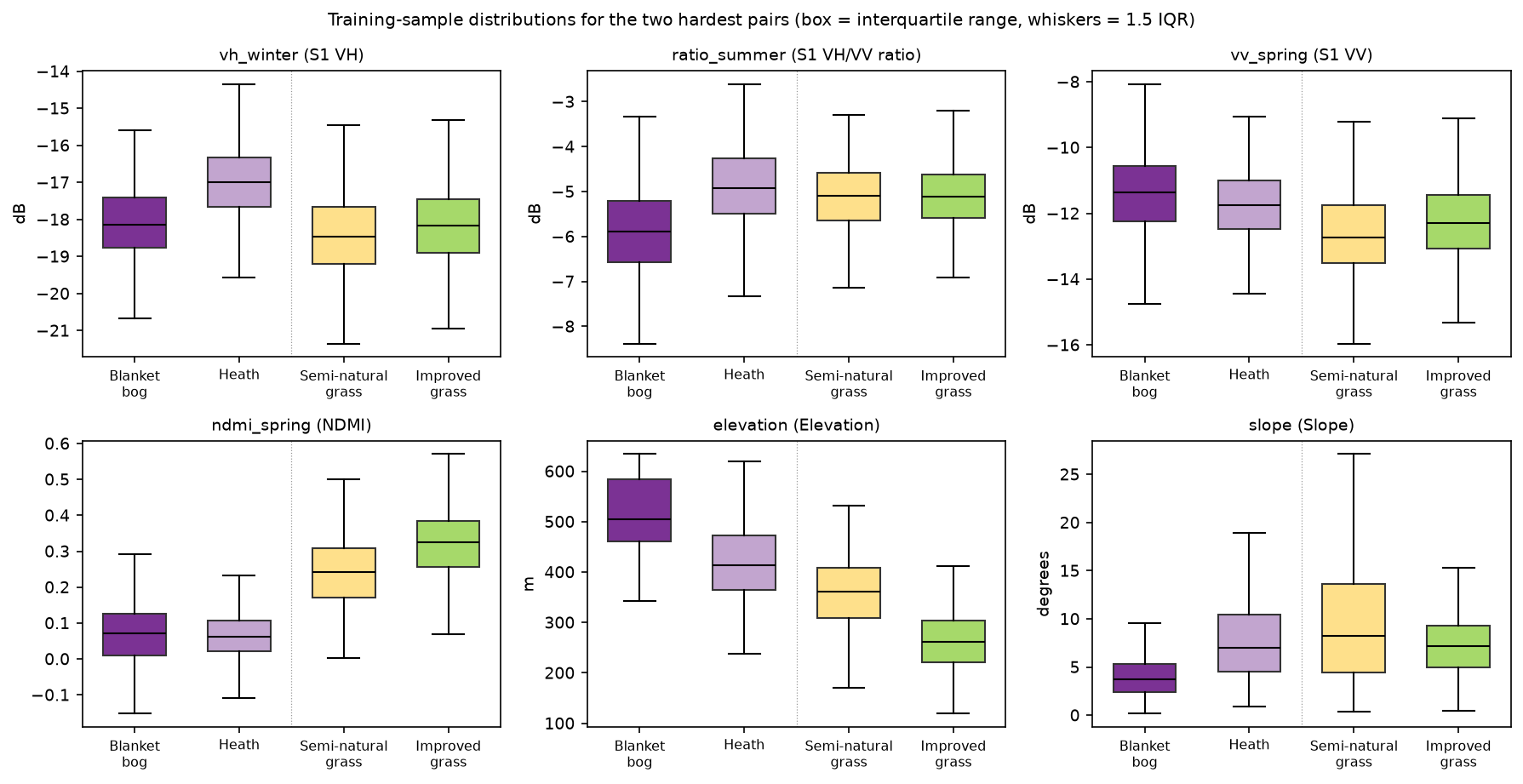
X_all = pd.DataFrame({k: hc.sample_values(v, samples) for k, v in FEAT.items()})y_all = samples["class_id"].to_numpy() - 1 # LightGBM wants classes 0..862 Sentinel-2 features (4 seasons x 10 bands + 5 indices, plus 2 NDVI change features)13 Sentinel-1 features (4 seasons x VV, VH, VH/VV in dB, plus the VH seasonal range)2 terrain features; elevation 115 to 635 m, slope median 7.3 degsample feature table: 9,000 x 77; share of missing values 0.69% (mostly winter Sentinel-2: LightGBM handles NaN natively)median of selected features by class (training samples only): bog heath brack semin impro broad conif water builtndre_summer 0.45 0.49 0.51 0.55 0.58 0.65 0.61 0.08 0.34ndmi_spring 0.07 0.06 -0.01 0.24 0.32 0.13 0.34 0.02 0.05vh_winter -18.15 -16.99 -15.39 -18.47 -18.17 -12.54 -13.45 -22.92 -13.39ratio_summer -5.89 -4.92 -6.05 -5.10 -5.11 -5.88 -5.08 -4.42 -6.17vv_spring -11.37 -11.74 -11.31 -12.72 -12.29 -7.70 -8.27 -18.83 -7.26elevation 504.73 413.70 328.72 360.96 261.89 244.12 324.08 211.00 188.84slope 3.75 6.99 15.87 8.24 7.13 12.99 14.22 0.00 4.17The medians already tell the story of the hard pairs. Bog and heath have almost the same NDMI, but heath is about 1.2 dB brighter in winter VH and 1 dB higher in the VH/VV ratio: the woody structure of heather scatters more cross-polarised energy than wet, mossy bog. Bog also lies higher (median 505 m against 414 m) and on gentler ground (3.7° against 7.0°). Semi-natural and improved grassland are nearly identical in radar. They differ in spring moisture (NDMI 0.24 against 0.32) and above all in elevation (361 m against 262 m), because farmers improve the grassland in the valleys and leave the high ground rough.
Step 3: class weights and tuning with spatial folds
The classes are balanced in the design, but a few samples fall on cloud gaps or block edges, so the training counts differ slightly. “Balanced” class weights, n ÷ (classes × class count), correct for that and make the method safe to reuse on unbalanced samples.
Tuning uses the five spatial folds of whole training blocks. A small grid of eight settings is enough: num_leaves controls tree complexity, min_data_in_leaf the smallest leaf and feature_fraction the share of features each tree may use. For every setting, lgb.cv trains with a learning rate of 0.05 and stops when the validation log loss has not improved for 100 rounds, so it returns the best number of trees as well.
counts = np.bincount(ytr, minlength=len(KEYS))cw = len(ytr) / (len(KEYS) * counts)            # "balanced" weights: n / (classes x class count)w_tr = cw[ytr]FOLDS = [(np.flatnonzero(fold != k), np.flatnonzero(fold == k)) for k in range(5)]BASE = {"objective": "multiclass", "num_class": len(KEYS), "learning_rate": 0.05, "bagging_fraction": 0.8,        "bagging_freq": 1, "lambda_l2": 1.0, "metric": "multi_logloss", "verbose": -1, "seed": hc.SEED,        "deterministic": True, "force_col_wise": True, "num_threads": 8}GRID = {"num_leaves": [15, 63], "min_data_in_leaf": [10, 40], "feature_fraction": [0.3, 0.7]}

def tune(cols):    """Grid search scored by blocked-CV log loss; early stopping picks the number of trees."""    rows = []    for vals in itertools.product(*GRID.values()):        p = {**BASE, **dict(zip(GRID, vals))}        ds = lgb.Dataset(Xtr[cols], ytr, weight=w_tr, free_raw_data=False)        cv = lgb.cv(p, ds, num_boost_round=3000, folds=FOLDS,                    callbacks=[lgb.early_stopping(100, verbose=False)])        loss = cv["valid multi_logloss-mean"]        rows.append({**dict(zip(GRID, vals)), "cv_logloss": loss[-1], "n_trees": len(loss)})    return pd.DataFrame(rows).sort_values("cv_logloss").reset_index(drop=True)
The script tunes each of the three feature sets separately, so the ablation compares well-tuned models rather than one setting that happens to suit the full stack.
class weights: bog 0.98, heath 1.08, brack 1.02, semin 1.15, impro 1.01, broad 1.06, conif 0.83, water 0.84, built 1.14
S2 (62 features): 8 settings tuned in 59 sbest: {'num_leaves': 15, 'min_data_in_leaf': 40, 'feature_fraction': 0.7}, 90 trees; blocked-CV log loss 0.4978, OA 0.831 +/- 0.020
S2+S1 (75 features): 8 settings tuned in 59 sbest: {'num_leaves': 15, 'min_data_in_leaf': 40, 'feature_fraction': 0.3}, 90 trees; blocked-CV log loss 0.4393, OA 0.848 +/- 0.015
S2+S1+terrain (77 features): 8 settings tuned in 55 s num_leaves  min_data_in_leaf  feature_fraction  cv_logloss  n_trees         15                40               0.3      0.3931       98         15                10               0.3      0.3951       95         63                40               0.3      0.3958       92         15                40               0.7      0.4026       86         63                40               0.7      0.4033       85         15                10               0.7      0.4069       86         63                10               0.3      0.4079       83         63                10               0.7      0.4214       70best: {'num_leaves': 15, 'min_data_in_leaf': 40, 'feature_fraction': 0.3}, 98 trees; blocked-CV log loss 0.3931, OA 0.867 +/- 0.022
same model, random 5-fold CV of the training samples: OA 0.894 (blocked 5-fold: 0.867)
Three things stand out. Small, conservative trees win: 15 leaves with at least 40 samples per leaf. With 6,544 samples from only 63 blocks, the model must not learn block-specific detail. A low feature_fraction of 0.3 suits the radar and terrain sets, because it forces trees to try features other than the dominant red-edge bands. And early stopping keeps only about 90 trees, so the whole tuning run takes about three minutes.
The last line repeats Part 1’s warning in a new form. The same model scored 89.4% with random 5-fold cross-validation and 86.7% with spatial folds. Random folds put validation pixels next to training pixels, so they reward memorising places. If you tune with random folds, you also pick settings that overfit to space.
Step 4: accuracy on the test blocks
Each tuned model is refitted on all training samples and applied once to the 2,456 test samples. Alongside the three LightGBM models are a scikit-learn random forest on the full 77 features (500 trees, balanced class weights) and Part 1’s rule-based map, sampled at the same test pixels.
for name, bb in best.items():    models[name] = fit(bb["cols"], bb["params"], bb["n_trees"])    preds[name] = models[name].predict(Xte[bb["cols"]]).argmax(1)
rf = RandomForestClassifier(n_estimators=500, class_weight="balanced", n_jobs=8, random_state=hc.SEED)rf.fit(Xtr[b["cols"]], ytr)                      # scikit-learn >= 1.4 forests accept NaN toopreds["Random forest"] = rf.predict(Xte[b["cols"]])
with rasterio.open(p1_tif) as src:               # Part 1's map, sampled at the same test pixels    p1_map = src.read(1)preds["Part 1 rules"] = hc.sample_values(p1_map, samples[~is_train]).astype(int) - 1
Every model is scored on the same pixels, so their differences can be tested with a paired block bootstrap. The script draws 2,000 resamples of the 27 test blocks once and reuses them for every model. A difference is then computed within each resample, which cancels most of the block-to-block variation that the models share.
UB = np.unique(test_blocks)BOOT = [np.concatenate([np.flatnonzero(test_blocks == bb) for bb in rng.choice(UB, UB.size, replace=True)])        for _ in range(2000)]                    # the same 2,000 block resamples for every model (paired)

def paired_diff(correct_a, correct_b): d = np.array([correct_a[i].mean() - correct_b[i].mean() for i in BOOT]) return correct_a.mean() - correct_b.mean(), np.percentile(d, [2.5, 97.5]), (d <= 0).mean()fit times: S2 0.5 s, S2+S1 0.4 s, S2+S1+terrain 0.4 s, Random forest 2.1 sPart 1 map sampled at the test pixels; unclassified there: 5 (scored as errors)test blocks: n = 2,456 samples in 27 blocks; 95% CI from 2,000 block-bootstrap resamples n_feat oa ci_lo ci_hi macro_f1 kappa f1_bog f1_heath f1_semin f1_impro bog<>heath semin<>impromodelPart 1: spectral rules 8 0.600 0.527 0.664 0.631 0.547 0.504 0.601 0.327 0.541 86 256Random forest (S2+S1+terrain) 77 0.831 0.758 0.883 0.840 0.808 0.837 0.849 0.606 0.714 58 192LightGBM: S2 62 0.790 0.718 0.848 0.805 0.761 0.787 0.807 0.529 0.628 73 238LightGBM: S2+S1 75 0.801 0.724 0.862 0.815 0.774 0.811 0.821 0.509 0.633 69 250LightGBM: S2+S1+terrain 77 0.853 0.801 0.892 0.862 0.833 0.862 0.841 0.703 0.753 59 155
paired block-bootstrap differences in overall accuracy (95% CI; share of resamples <= 0): LightGBM: S2+S1 - LightGBM: S2 +0.011 (-0.001 to +0.026; 0.043) LightGBM: S2+S1+terrain - LightGBM: S2+S1 +0.052 (+0.022 to +0.092; 0.000) LightGBM: S2+S1+terrain - LightGBM: S2 +0.064 (+0.035 to +0.101; 0.000) LightGBM: S2+S1+terrain - Random forest (S2+S1+terrain) +0.023 (+0.003 to +0.048; 0.009) LightGBM: S2 - Part 1: spectral rules +0.190 (+0.159 to +0.220; 0.000) LightGBM: S2+S1+terrain - Part 1: spectral rules +0.254 (+0.209 to +0.305; 0.000)Part 1’s map scores 60.0% here, matching Part 1’s own assessment. Its macro F1 is 0.631 rather than 0.630 because five test pixels fall on map pixels left unclassified, which count as errors.
What Sentinel-1 adds: bog versus heath, and the grasslands
Machine learning alone is the biggest step. LightGBM on Sentinel-2 alone scored 79.0%, 19 points above the rules on the same imagery, because it can use all 62 bands and indices across four seasons rather than eight thresholds.
Adding Sentinel-1 helps less than you might expect: +1.1 points, with a 95% interval of −0.1 to +2.6. The gain is in the place the medians predicted. Bog F1 rose from 0.787 to 0.811, heath from 0.807 to 0.821, and bog–heath confusions fell from 73 to 69. Radar sees the structural difference between heather and wet bog that optical bands blur. For the grasslands, radar did nothing useful: semi-natural grassland F1 fell slightly from 0.529 to 0.509 and the grassland confusions rose from 238 to 250. Both are short, closed swards that scatter C-band radar in much the same way.
Cross-validation showed a larger radar gain than the test blocks did: log loss fell from 0.498 to 0.439 and CV accuracy rose from 83.1% to 84.8%. The test set has only 27 blocks, so some of this gap is chance. A fair summary is that Sentinel-1 gives a small, consistent improvement for the moorland classes in a region where Sentinel-2 already has good cloud-free composites. It would matter more where clouds leave optical gaps.
Terrain: the biggest single gain
Adding just two terrain features gave +5.2 points (+2.2 to +9.2), more than radar. Grassland confusions dropped from 250 to 155, semi-natural grassland F1 from 0.509 to 0.703, and bog–heath confusions from 69 to 59. Blanket bog needs high rainfall and gentle slopes to form deep peat, and improved grassland sits on the lower, farmed valley sides, so elevation and slope are real ecological signals.
Be careful with that result, though. Elevation is also a location proxy: within one 25 km study area it can stand in for “which valley”, which helps the model reproduce Living England’s local patterns without learning anything that transfers. The Copernicus DEM is also a surface model, so woodland canopies and buildings raise its elevation. Test terrain features again before trusting them in a different landscape.
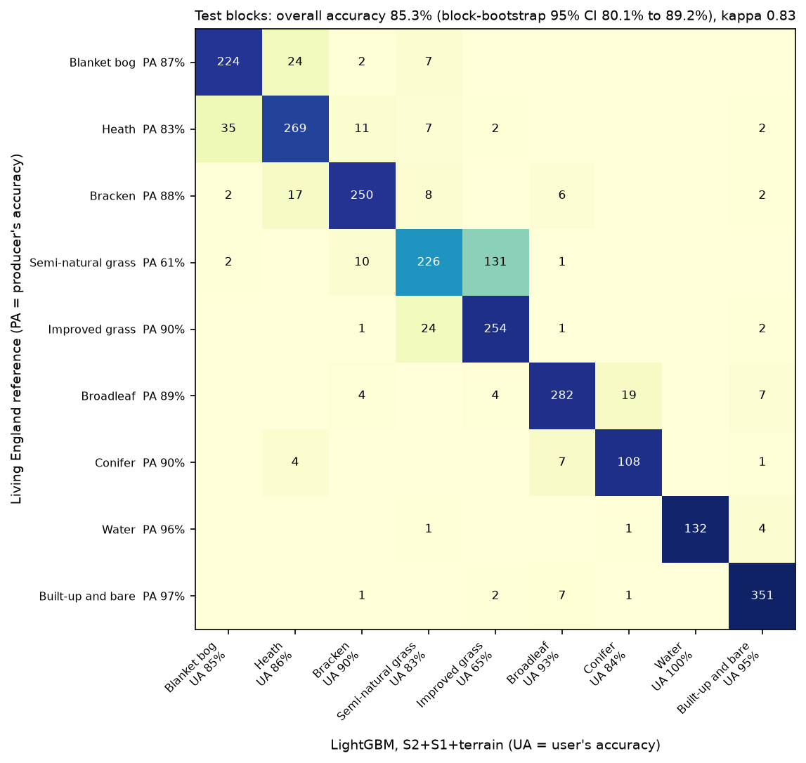
n_test producers_acc users_acc f1 f1_part1Blanket bog 257 0.872 0.852 0.862 0.504Heath 326 0.825 0.857 0.841 0.601Bracken 285 0.877 0.896 0.887 0.649Semi-natural grassland 370 0.611 0.828 0.703 0.327Improved grassland 282 0.901 0.646 0.753 0.541Broadleaf woodland 316 0.892 0.928 0.910 0.660Conifer woodland 120 0.900 0.837 0.867 0.805Water 138 0.957 1.000 0.978 0.891Built-up and bare 362 0.970 0.951 0.960 0.697overall accuracy 0.853 (block-bootstrap 95% CI 0.801 to 0.892); macro F1 0.862; kappa 0.833Every class improves on Part 1, and blanket bog improves the most (F1 0.50 to 0.86). Semi-natural grassland is still the weak spot: 131 of its 370 test samples were called improved grassland, so improved grassland is over-mapped (user’s accuracy 65%). The two classes are a continuum of management intensity, and Living England’s boundary between them is itself uncertain.
Against a random forest
The random forest on the same 77 features scored 83.1%, so LightGBM is 2.3 points better (paired 95% CI +0.3 to +4.8). That is a real but modest edge. The forest even matched LightGBM on heath and bog–heath confusions; its losses were in the grasslands. Note too that the random forest with radar and terrain (83.1%) beat LightGBM without terrain (80.1%). Feature engineering mattered more than the choice of algorithm, a pattern you will also see in the random forest land cover tutorial.
Step 5: what the model uses
Gain importance, the total loss reduction from splits on each feature, is free but biased towards features with many distinct values. Two better tools are TreeSHAP, which LightGBM computes exactly, and permutation importance on the test blocks.
contrib = model.predict(Xte[cols], pred_contrib=True).reshape(len(Xte), len(KEYS), len(cols) + 1)[:, :, :-1]shap_abs = pd.DataFrame(np.abs(contrib).mean(0).T, index=cols, columns=KEYS) # mean |SHAP| per classbh = np.isin(yte, [I["bog"], I["heath"]])bog_vs_heath = pd.Series(np.abs(contrib[bh, I["bog"], :] - contrib[bh, I["heath"], :]).mean(0), index=cols)For a multiclass model, pred_contrib=True returns one block of SHAP values per class plus a bias column, in log-odds. The last line asks a sharper question: on bog and heath test samples, which features push the bog score and the heath score apart?
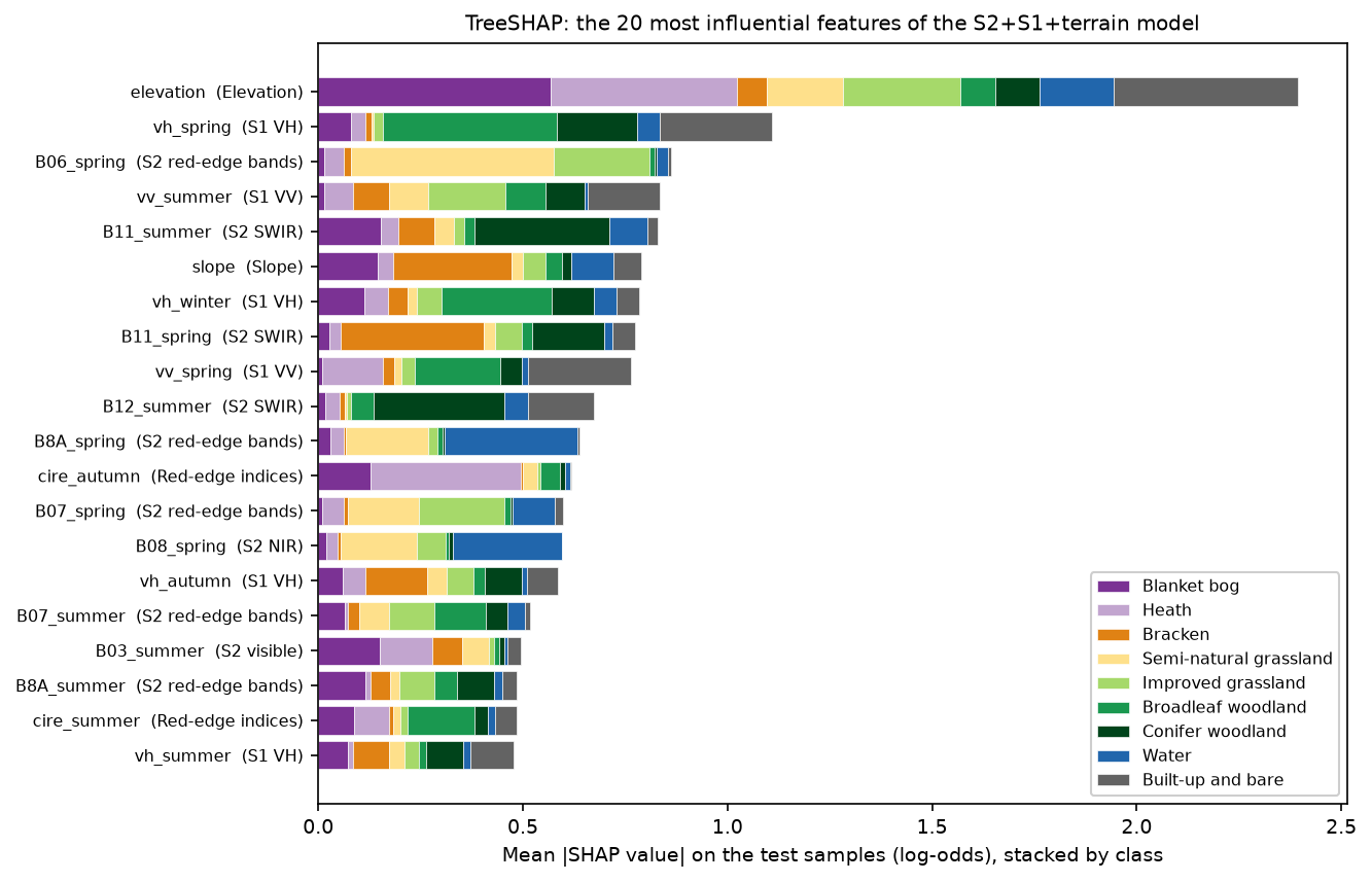
top 12 features by mean |SHAP| (summed over classes):elevation 2.395vh_spring 1.109B06_spring 0.861vv_summer 0.834B11_summer 0.830slope 0.789vh_winter 0.784B11_spring 0.775vv_spring 0.764B12_summer 0.673B8A_spring 0.639cire_autumn 0.619top 8 features separating bog from heath (mean |SHAP(bog) - SHAP(heath)| on bog and heath test samples):elevation 0.830B11_summer 0.247cire_autumn 0.243slope 0.225B03_spring 0.208B04_spring 0.205cire_spring 0.193ratio_spring 0.184Elevation is the most used feature overall and by far the most important for separating bog from heath. After it come summer SWIR (moisture), the autumn red-edge chlorophyll index (which mainly drives the heath score), slope, spring visible bands and the spring VH/VV ratio. Radar appears high in the overall ranking, mostly for woodland and built-up land, where VH and VV are very different from open ground.
SHAP describes how the model uses a feature, not how much accuracy depends on it. Correlated features share the credit, and a feature can be used heavily even when a near-copy could replace it. Permutation importance answers the second question. Because seasonal bands are strongly correlated, the script shuffles whole groups of features together, such as all 16 red-edge band features, and records the drop in test macro F1 over ten repeats:
for g in groups: gcols = [c for c in cols if GROUP[c] == g] drops = [] for _ in range(N_REP): Xp = Xte[cols].copy() Xp[gcols] = Xp[gcols].to_numpy()[prng.permutation(len(Xp))] # shuffle the group's rows together drops.append(base_f1 - summarise(yte, model.predict(Xp).argmax(1))["macro_f1"]) perm[g] = (np.mean(drops), np.std(drops), len(gcols))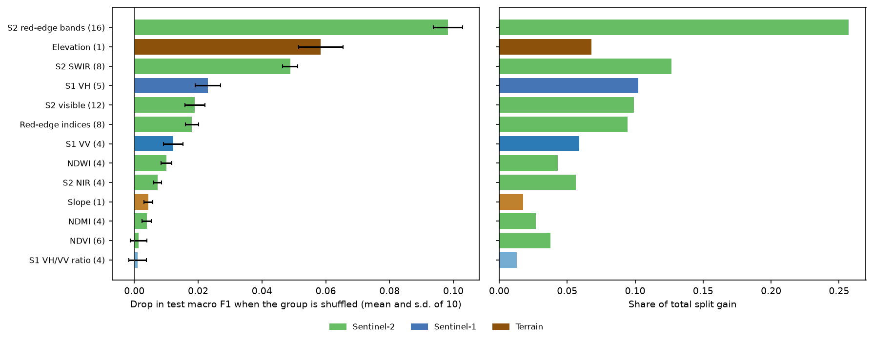
The red-edge bands are the group the model can least do without (macro F1 drops by 0.098 when shuffled), followed by elevation (0.058) and SWIR (0.049). VH is the most useful radar group (0.023). NDVI and the VH/VV ratio barely matter, not because they carry no signal, but because the model can rebuild it from the raw bands they are computed from. Slope looks unimportant here (0.004) although it ranked sixth by SHAP: with elevation and the red-edge bands present, little of its information is unique.
Step 6: the whole map and its confidence
The model predicts the 5.6 million pixels of the grid in chunks of 250 rows, and keeps the top-class probability as a confidence layer. Pixels without a clear spring or summer view would be left unclassified; in 2023 there were virtually none.
for r0 in range(0, rows_, STEP): Xc = np.stack([FEAT[c][r0:r0 + STEP].ravel() for c in cols], axis=1) p = model.predict(Xc) pred_map[r0:r0 + STEP] = (p.argmax(1) + 1).reshape(-1, cols_) conf_map[r0:r0 + STEP] = p.max(1).reshape(-1, cols_)hc.write_geotiff(OUT / "habitat_lightgbm_2023.tif", pred_map, nodata=0)hc.write_geotiff(OUT / "habitat_lightgbm_confidence_2023.tif", conf_map, nodata=np.nan, dtype="float32")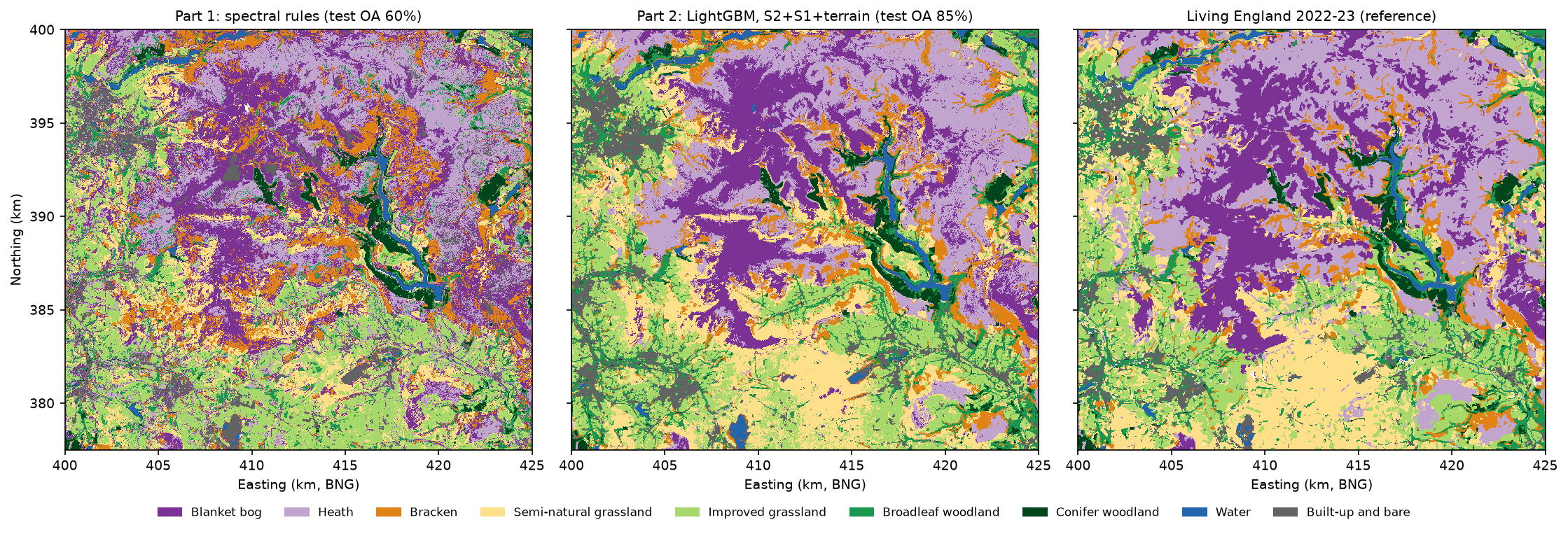
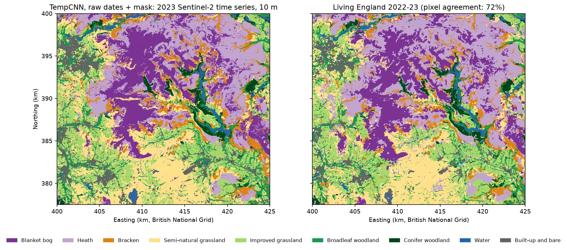
predicted 5,625,000 pixels in 10 s; unclassified (no clear spring or summer view): 0.00% lightgbm_km2 part1_km2 living_england_km2Blanket bog 86.2 131.0 90.5Heath 122.9 109.9 151.5Bracken 52.2 64.1 41.6Semi-natural grassland 99.0 63.5 96.1Improved grassland 97.1 101.9 90.0Broadleaf woodland 44.0 35.4 39.7Conifer woodland 16.6 17.3 17.2Water 8.8 6.3 8.4Built-up and bare 35.7 32.9 25.7wall-to-wall agreement with Living England, LightGBM: test blocks 0.687, whole area 0.690wall-to-wall agreement with Living England, Part 1 rules: test blocks 0.483, whole area 0.490 pixels with top-class probability 0.0-0.5: 9.0% of the map, agreement 0.342 pixels with top-class probability 0.5-0.8: 31.1% of the map, agreement 0.530 pixels with top-class probability 0.8-1.0: 59.9% of the map, agreement 0.826The class areas are now close to Living England’s for bog (86 against 91 km²) and semi-natural grassland (99 against 96 km²), where Part 1 was far off. Heath is still under-mapped by 29 km²; on the test samples it was most often confused with bog.
Pixel-by-pixel agreement with Living England over the whole area is 69%, against 85% on the test samples. The gap is the cost of pure samples: the full map includes mixed pixels, field edges, transitions between habitats and lower-reliability polygons. Part 1 shows the same gap (49% against 60%). Use sample accuracy to compare methods and wall-to-wall agreement to judge the map. Part 5 returns to this with area-adjusted accuracy.
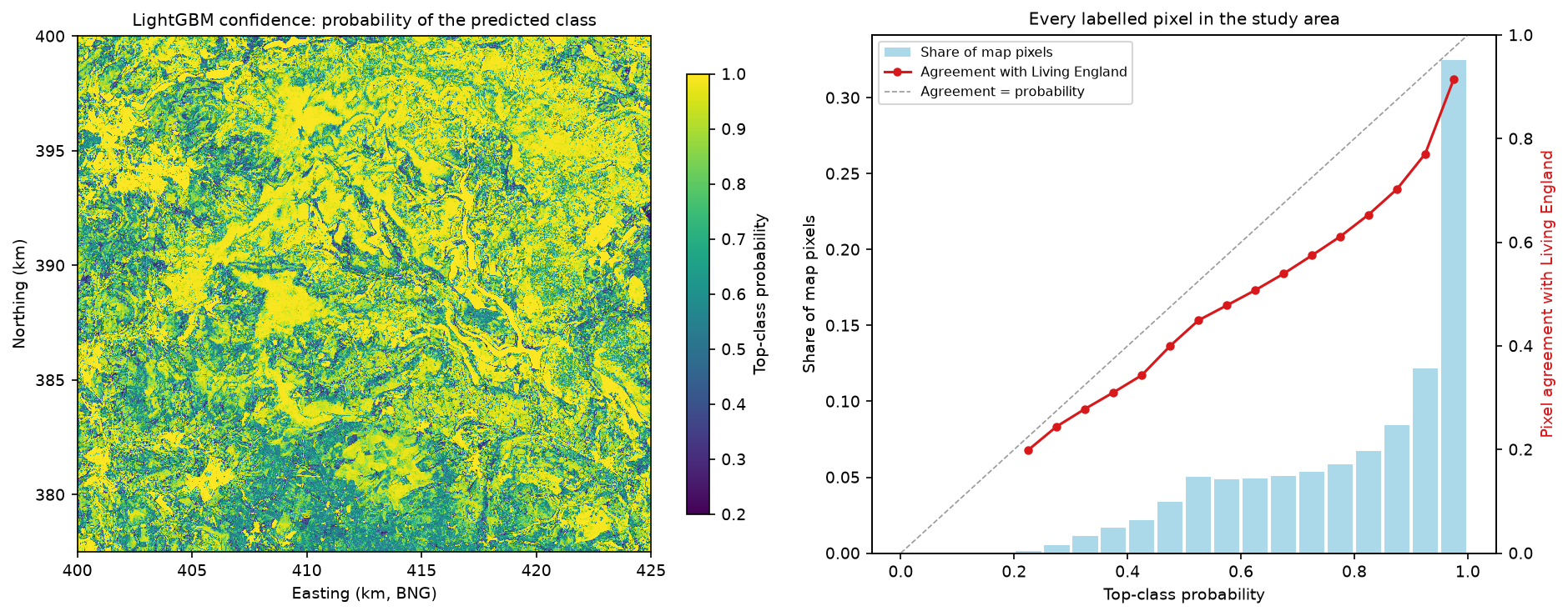
The confidence layer is useful. Sixty per cent of the map has a top-class probability of at least 0.8, and there the agreement is 83%; in the 9% of pixels below 0.5 it is only 34%. Low confidence picks out the grassland mosaics of the valleys and the edges between habitats. But the probabilities are over-confident for wall-to-wall pixels, because the model was trained on pure samples. Treat them as a ranking for where to check the map, not as calibrated probabilities. Part 5 covers uncertainty properly.
Results so far in the series
| Method | Features | Test OA (95% CI) | Macro F1 | Kappa | Map agreement |
|---|---|---|---|---|---|
| Part 1: spectral rules | 8 indices | 60.0% (52.7–66.4) | 0.63 | 0.55 | 49.0% |
| Random forest | 77 (S2+S1+terrain) | 83.1% (75.8–88.3) | 0.84 | 0.81 | — |
| LightGBM, S2 | 62 | 79.0% (71.8–84.8) | 0.81 | 0.76 | — |
| LightGBM, S2+S1 | 75 | 80.1% (72.4–86.2) | 0.82 | 0.77 | — |
| LightGBM, S2+S1+terrain | 77 | 85.3% (80.1–89.2) | 0.86 | 0.83 | 69.0% |
All rows use the identical 2,456 test pixels in 27 blocks. The headline model, LightGBM with S2+S1+terrain, is the number Parts 3 to 5 have to beat. In the event, none of them beats it by more than the uncertainty: see the five-method comparison in Part 5. The whole script runs in about three minutes on 8 CPU threads once the composites are cached.
Limitations
- The labels are a model. Living England was built from Sentinel-1, Sentinel-2 and ancillary data, so a model on similar inputs can partly reproduce its method rather than the habitats on the ground. Agreement above about 85% would be hard to interpret.
- Balanced, pure samples flatter the score. The test samples come from homogeneous, high-reliability polygons with equal numbers per class. The wall-to-wall agreement of 69% is the more realistic figure for the map as a whole.
- Elevation is partly a location proxy. Its large gain may not transfer to another upland. The Copernicus DEM is a surface model at 30 m, resampled to 10 m, so slope is smoothed and woodland and buildings are raised.
- Seasonal medians hide timing. Four composites per sensor throw away the date of green-up and senescence and the radar response to individual rain events. Part 4 uses the full time series instead.
- Modest tuning. Eight settings and early stopping were enough here, with all three feature sets choosing similar small trees. A larger search might add a point, at the risk of overfitting the five folds.
- One year, one area. All results are for 2023 in the Dark Peak. Validate on another year or region before reusing the model.
Try it yourself
- Radar alone. Add
"S1": S1_COLSand"S1+terrain": S1_COLS + TERRAIN_COLStoFEATURE_SETS. How far does cloud-free radar get without any optical data, and which classes collapse? - Terrain without location. Replace elevation with features that describe shape rather than height, such as slope, aspect and the topographic position index from raster terrain analysis with rasterio. Does the grassland gain survive?
- One orbit direction. Rebuild the Sentinel-1 composites with
hc.s1_composite(s, m, orbit_state="descending")and compare with the mixed-orbit version. Look-direction effects on steep valley sides are a common source of radar error. - No class weights. Set
w_trto ones, retune and compare user’s and producer’s accuracy for the smallest training class, conifer woodland. - Calibrate the confidence. Fit isotonic regression of “agrees with Living England” against top-class probability on the training blocks, then check whether the calibrated probabilities lie on the diagonal for the test blocks.
Frequently asked questions
Is LightGBM better than random forest for land cover classification?
Usually a little, and here by 2.3 percentage points of overall accuracy on the same 77 features (85.3% against 83.1%, paired 95% CI +0.3 to +4.8). LightGBM also trained five times faster, handled missing values natively and gave exact SHAP values for free. A random forest needs almost no tuning, though, and adding better features helped more than switching algorithm. Both are good choices; test them on the same spatial split.
Does Sentinel-1 improve Sentinel-2 land cover classification?
It helps most where the classes differ in structure or wetness rather than colour, or where clouds leave gaps in the optical data. In the Dark Peak, adding seasonal VV, VH and the VH/VV ratio to good Sentinel-2 composites raised overall accuracy by only 1.1 points. It did improve bog and heath, because heather scatters more cross-polarised radar than wet bog. It did not help separate semi-natural from improved grassland.
How do I do spatial cross-validation with LightGBM?
Assign each training sample to a fold by the spatial block it falls in, then pass the folds to lgb.cv as a list of (train_indices, validation_indices) pairs through the folds argument. Add lgb.early_stopping so that each setting also finds its best number of trees. In this tutorial random folds reported 89.4% accuracy for a model that scored 86.7% with spatial folds and 85.3% on separate test blocks.
Should I use SHAP or permutation importance?
Use both, because they answer different questions. SHAP shows how the model uses each feature for each class and each pixel, which is good for understanding decisions such as bog versus heath. Permutation importance on held-out data shows how much accuracy depends on a feature. With correlated features, such as seasonal bands, permute whole groups of features together, or the importance is spread thinly across near-copies.
Does LightGBM handle missing values from clouds?
Yes. LightGBM treats NaN as missing and learns at every split which side missing values should go to, so pixels with no clear winter view can still be classified from their other seasons. You do not need to gap-fill or drop them. Make sure infinite values, for example from dividing by zero in an index, are converted to NaN first.
Should I add a DEM to a habitat classification?
In uplands, usually yes: elevation and slope gave the largest single gain here, 5.2 points of overall accuracy, and cut the confusion between semi-natural and improved grassland by more than a third. Check that the gain is ecological rather than geographic, though. Within a small area elevation can act as a proxy for location, and that does not transfer to other regions.
Next steps
- Start the series from Part 1: habitat mapping with Sentinel-2 in Python for the rule-based baseline, the accuracy assessment and why random splits overstate accuracy.
- Compare with a global-label workflow in Land cover classification with a Sentinel-2 random forest.
- Learn more about the radar features in SAR speckle filtering in Python, Sentinel-1 crop monitoring and Sentinel-1 SAR flood mapping.
- Improve the optical inputs with Sentinel-2 cloud masking in Python and NDVI time series with odc-stac.
- Summarise the habitat map by moorland unit or catchment with zonal statistics in Python.
- Continue the series: Part 3 turns the pixels into image objects and classifies those instead, Part 4 trains TempCNN and L-TAE on the full Sentinel-2 time series, and Part 5 maps the same habitats from AlphaEarth embeddings with a fraction of the labels.
Data and licences
- Living England Habitat Map 2022-23: © Natural England, under the Open Government Licence v3.0. Contains Ordnance Survey data © Crown copyright and database right. Accessed from Natural England’s public ArcGIS service on 21 October 2026.
- Sentinel-2 L2A: contains modified Copernicus Sentinel data 2023, free and open under the Copernicus data licence. Accessed from the Microsoft Planetary Computer.
- Sentinel-1 RTC: contains modified Copernicus Sentinel data 2023, processed by ESA; radiometric terrain correction by Catalyst/Microsoft. Licensed CC BY 4.0. Accessed from the Microsoft Planetary Computer.
- Copernicus DEM GLO-30: © DLR e.V. 2010-2014 and © Airbus Defence and Space GmbH 2014-2018, provided under COPERNICUS by the European Union and ESA; all rights reserved. Free to use under the Copernicus DEM licence. Accessed from the Microsoft Planetary Computer on 21 October 2026.
- References: Ke, G. et al. (2017), “LightGBM: a highly efficient gradient boosting decision tree”, Advances in Neural Information Processing Systems 30. Lundberg, S. M. et al. (2020), “From local explanations to global understanding with explainable AI for trees”, Nature Machine Intelligence 2, 56–67. Roberts, D. R. et al. (2017), “Cross-validation strategies for data with temporal, spatial, hierarchical, or phylogenetic structure”, Ecography 40(8), 913–929.
- Code:
habitat_lightgbm.pyand the shared series module (habitat_common.py,prepare_data.py, sample CSVs), tested with Python 3.12.0, LightGBM 4.7.0, scikit-learn 1.9.1, NumPy 2.5.4, pandas 3.0.6, odc-stac 0.5.3 and rasterio 1.5.2.
Key terms
- LightGBM
- A fast open-source gradient boosting library from Microsoft. It builds an ensemble of small decision trees, each correcting the errors of the trees before it, and handles missing values natively.
- Gradient boosting
- A way of building a model from many weak learners, usually shallow trees, added one at a time so that each new tree reduces the remaining error of the ensemble.
- Data fusion
- Combining measurements from different sensors, here optical Sentinel-2, radar Sentinel-1 and a digital elevation model, into one feature table for a single classifier.
- Spatial cross-validation
- Cross-validation in which the folds are groups of whole spatial blocks rather than random samples, so that validation pixels are never next to training pixels.
- Ablation study
- Measuring what each part of a model contributes by removing it, here by training the same classifier on growing sets of features.
- SHAP value
- A feature's additive contribution to one prediction, from Shapley values in game theory. TreeSHAP computes them exactly and quickly for tree ensembles.
- Permutation importance
- The drop in a model's test score when the values of one feature, or one group of features, are randomly shuffled between samples.
Data for this tutorial
- Living England Habitat Map · Natural England's broad habitat map, used as labels (2022-23 release)
- Microsoft Planetary Computer · Sentinel-2 L2A, Sentinel-1 RTC and Copernicus DEM through STAC, no account needed
- Copernicus DEM GLO-30 · 30 m global surface model, used for elevation and slope
Licences and formats for each source are listed in the GIS data sources catalogue.