Satellite image time series classification with deep learning: TempCNN and L-TAE in PyTorch on a CPU
Classify habitats from a full year of cloudy, irregular Sentinel-2 observations with two temporal neural networks in PyTorch: a 1D convolutional TempCNN and a lightweight temporal attention encoder (L-TAE) with day-of-year positional encoding. Compare masking with gap-filling, test against a LightGBM baseline on spatial blocks, read which dates matter from attention and occlusion, and predict a wall-to-wall 10 m map on a CPU.
- Level
- Advanced
- Tested with
- Python 3.12
- Source code
- Download scripts
Key takeaways
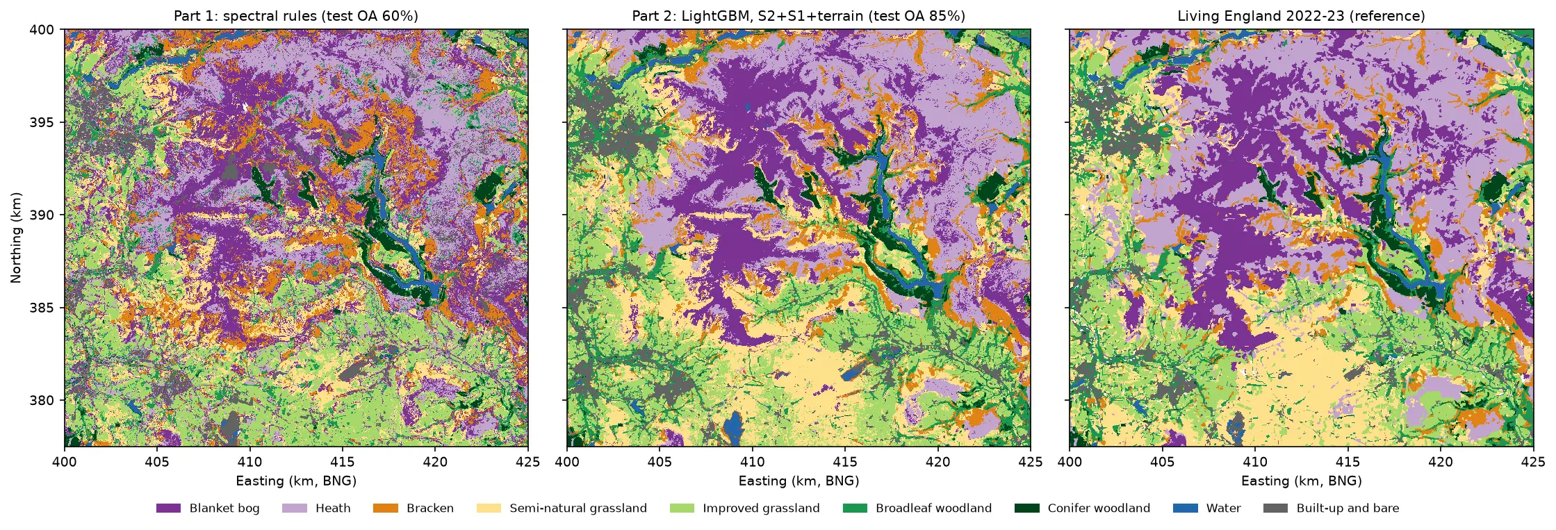
- A TempCNN fed each pixel's 50 raw, cloudy Sentinel-2 dates plus a clear-sky mask reaches 85.1% overall accuracy on the series' held-out spatial blocks (block-bootstrap 95% CI 81.1% to 88.4%), macro F1 0.86 and kappa 0.83, against 60.0% for the Part 1 spectral rules.
- LightGBM on the same per-date values scores 84.2%. The deep model's lead of 0.9 points has a paired 95% interval of −0.7 to +2.9 points, so on this data it is not a significant win.
- Feeding the raw dates with a mask beat linear gap-filling onto a 10-day grid for every model, by 0.9 to 4.4 points. The L-TAE, with 44,000 parameters and a day-of-year encoding, scored best on test (86.5%) and lost least when clear views were removed.
- Attention peaks in early April, late May and early September; hiding June costs the most accuracy. The 10 m wall-to-wall map agrees with Living England on 70% of the test blocks, up from 48% for the rules.
Before you start
- Confident Python with NumPy and pandas, and the basics of PyTorch (tensors, nn.Module, a training loop); training a U-Net in PyTorch is a good warm-up
- Part 1 of this series for the study area, labels, classes and the spatial train/test split
- Python 3.12 with the series' shared environment plus CPU PyTorch 2.14 and LightGBM 4.7 (see requirements.txt)
- About 8 GB of free disk space for the full-area image stack, 16 GB of RAM and an internet connection; no GPU, account or API key needed
Short answer: to classify a satellite image time series with deep learning, give the network every observation of each pixel through the year, with its date and a flag for whether it was clear. Do not reduce the year to a few composites first. A 1D convolutional network (TempCNN) or a small attention model with a day-of-year positional encoding (L-TAE) trains on 6,500 labelled pixels in a few minutes on a laptop CPU. In the Dark Peak, a TempCNN on 50 raw, cloudy Sentinel-2 dates maps nine habitats with 85% overall accuracy on held-out spatial blocks. That is 25 points better than the spectral rules of Part 1. But LightGBM on the same inputs reaches 84%, so a well-tuned tree model remains a strong rival.
Part 1 of this series reduced 2023 to seasonal composites and classified them with eight threshold rules. That throws away most of the year: the timing of green-up, the bracken canopy unfurling in June, the heather browning in autumn. This part keeps every date. Each pixel becomes a sequence of up to 50 Sentinel-2 spectra, and a neural network learns which parts of the sequence separate blanket bog from heath and semi-natural from improved grassland.
The catch is clouds. Over the Peak District only 39% of the observations are clear, and each pixel is clear on a different set of dates. Most of this tutorial is about how to deal with that.
This is part 4 of a five-part series, AI habitat classification with Python. Every part uses the same study area, labels, class scheme and train/test split:
- Part 1: rule-based habitat mapping with Sentinel-2 and an honest accuracy assessment. Its numbers are the baseline.
- Part 2: machine learning on multi-temporal Sentinel-2 and Sentinel-1 features with LightGBM.
- Part 3: object-based image analysis (OBIA).
- Part 4 (this tutorial): deep learning on the full time series, in PyTorch on a CPU.
- Part 5: foundation models, few-shot learning, uncertainty and area-adjusted accuracy.
This part does not need Parts 2 or 3. It trains its own LightGBM baseline so that the deep models have a fair, like-for-like comparison.
You will learn how to:
- turn a cloudy Sentinel-2 archive into per-pixel time series with a clear-sky mask;
- handle irregular dates in two ways, masking with day-of-year encoding and gap-filling onto a regular grid;
- write a TempCNN and a lightweight temporal attention encoder in plain PyTorch, and see the equations behind attention;
- train with spatial folds for early stopping, fixed seeds and observation-dropout augmentation;
- compare honestly with a LightGBM baseline, using a paired block bootstrap;
- find which dates matter with attention weights and occlusion;
- predict a wall-to-wall 10 m map from a 5.6 GB stack on a CPU.
All outputs below come from habitat_time_series_dl.py and the series’ shared module and sample design (habitat_common.py, prepare_data.py and the sample CSVs). They were run on 21 October 2026 with Python 3.12, PyTorch 2.14.1 (CPU build), LightGBM 4.7.0, NumPy 2.5.4 and pandas 3.0.6 on 8 CPU threads, with no GPU. Training all 18 models took 8 minutes, and the full script took about 19 minutes, including the image download.
Spatial CNN or temporal model?
If you followed Train a U-Net for satellite image segmentation, you have already trained a convolutional network on Sentinel-2. That U-Net is a spatial model: it looks at a 2D chip of one composite image and learns shapes, edges and texture. The models here are temporal: they look at one pixel at a time, but at every date of the year. The convolution in TempCNN runs along time, not across space.
The two views suit different problems. Buildings, roads and field boundaries are defined by shape, so a spatial model wins. Habitats in the uplands often look alike on any one day and differ mostly in when they green up and brown off, so the time series carries most of the signal. The two can be combined (U-TAE, Garnot and Landrieu 2021, is a U-Net with temporal attention), but that needs far more memory and usually a GPU.
Install PyTorch for CPU
Use the series’ shared environment, then add the CPU build of PyTorch from the PyTorch index and LightGBM. On Linux, the default PyTorch wheels bundle CUDA and are several gigabytes; the CPU wheel is about 200 MB.
python -m venv .venv-habitat.venv-habitat\Scripts\Activate.ps1pip install torch==2.14.1 --index-url https://download.pytorch.org/whl/cpupip install -r tutorial-code\satellite-image-time-series-deep-learning-pytorch\requirements.txtOn macOS or Linux, activate with source .venv-habitat/bin/activate and use forward slashes. The requirements file pulls in the shared pins (odc-stac, rasterio, geopandas, pandas and so on) and adds lightgbm==4.7.0.
Step 1: the irregular, cloudy time series
You do not need to have run Parts 1 to 3. The shared module builds this part’s inputs with one command. It reads the committed sample design (9,000 pixels, 1,000 per class, 27 test blocks), finds every 2023 Sentinel-2 date with at least 5% of the area clear, and samples the ten 10 m and 20 m bands at each pixel on each date, together with a clear flag from the scene classification layer.
cd tutorial-code\satellite-image-time-series-deep-learning-pytorchpython ..\ai-habitat-classification-common\prepare_data.py --timeseries # about 5 minutes, oncepython habitat_time_series_dl.pyThe script reshapes the long table into three arrays: reflectance X (samples × dates × bands, NaN where cloudy), the clear mask M and the labels y. Each band is then standardised with the mean and standard deviation of clear training observations only, so nothing from the test blocks leaks into the inputs.
import habitat_common as hc
samples = hc.load_samples().sort_values("sample_id").reset_index(drop=True)ts = hc.s2_sample_timeseries().sort_values(["sample_id", "date"])dates = pd.DatetimeIndex(np.sort(ts["date"].unique()))DOY = dates.dayofyear.to_numpy().astype("float32")N, T, C = len(samples), len(dates), len(BANDS)X = ts[BANDS].to_numpy("float32").reshape(N, T, C)      # reflectance, NaN where cloudyM = ts["clear"].to_numpy(bool).reshape(N, T)            # True where the pixel was clear on that datey = samples["class_id"].to_numpy() - 1                  # 0..8
mu = np.nanmean(X[is_train].reshape(-1, C), axis=0) # clear training observations onlysd = np.nanstd(X[is_train].reshape(-1, C), axis=0)XN = np.nan_to_num((X - mu) / sd, nan=0.0).astype("float32") # cloudy -> 0 (the training mean)9,000 samples x 50 dates x 10 bands; 39.5% of observations clearclear dates per sample: median 20, 10th percentile 14, min 2, max 35; 4 samples have fewer than 5longest gap between clear views: median 58 days, 90th percentile 80 daysshare of sample observations clear, by month: Jan 25%, Feb 39%, Mar 47%, Apr 51%, May 34%, Jun 69%, Jul 18%, Aug 23%, Sep 48%, Oct 22%, Nov 33%, Dec 39%A typical pixel has 20 clear views out of 50, and its longest run without one is about two months. July and August, the height of summer, are mostly cloudy. June 2023 was unusually sunny, so it holds a large share of the clear views.
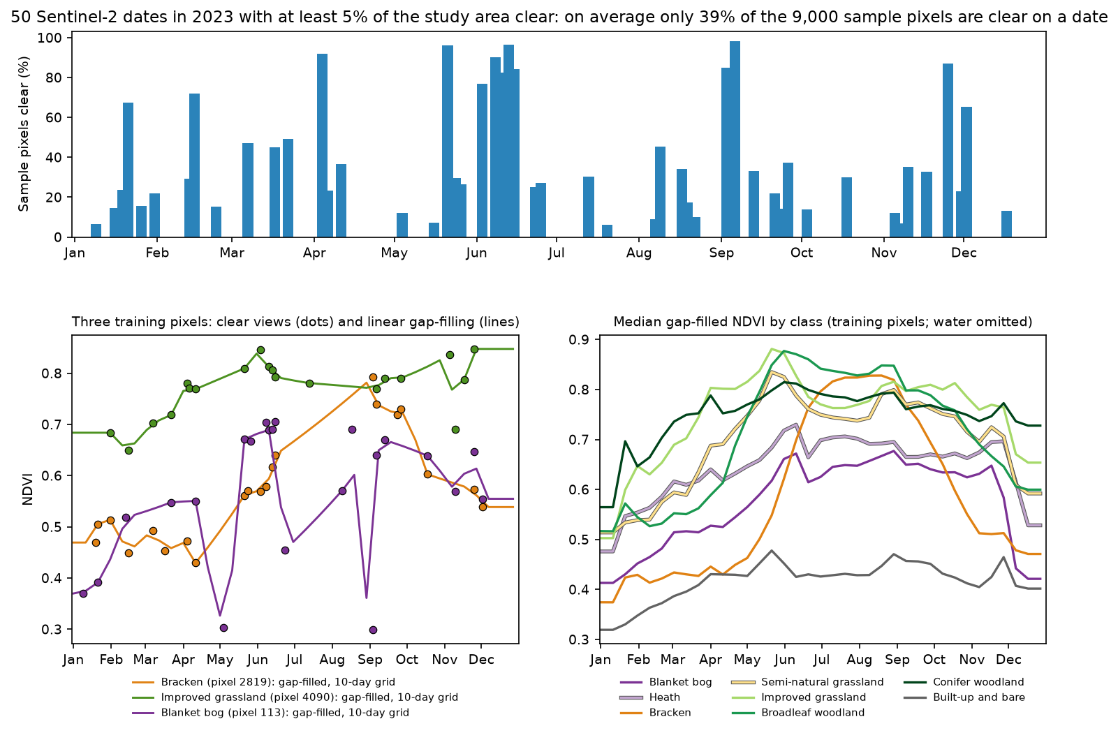
The class curves show why a time series helps. Bracken is the lowest vegetated class in April and among the highest in August. Improved grassland greens up a month before semi-natural grassland. Bog and heath run parallel, with bog lower all year, which hints that they will stay hard to separate.
Step 2: two ways to handle cloud gaps
A neural network needs a fixed-size input, but each pixel has clear views on different dates. There are two common answers.
Gap-filling. Interpolate each pixel’s clear observations onto a regular grid, here every 10 days from 1 January (37 steps), repeating the nearest clear value before the first and after the last view. Every pixel then has the same, complete input, and any model works. The cost is that interpolated values are invented. A 58-day gap is bridged by a straight line, and the model cannot tell real values from guesses.
Masking. Keep all 50 acquisition dates, set cloudy values to zero, and pass the clear mask alongside. The model sees only real observations and knows which are missing. For TempCNN the mask becomes an 11th input channel. For the attention model, cloudy dates are excluded from the softmax, so they get exactly zero weight.
The gap-filling is vectorised, with no Python loop over pixels. For each grid day it finds the last clear view on or before it and the first after it, and interpolates linearly between them:
GRID = np.arange(1, 366, 10)             # regular 10-day day-of-year grid (37 steps)
def gapfill(xn, m, t_obs=DOY, t_grid=GRID):    n, nt = m.shape    ar = np.arange(nt)    prev = np.maximum.accumulate(np.where(m, ar, -1), axis=1)                       # last clear index <= t    nxt = np.minimum.accumulate(np.where(m, ar, nt)[:, ::-1], axis=1)[:, ::-1]      # first clear index >= t    j = np.searchsorted(t_obs, t_grid, side="right")    p = np.concatenate([np.full((n, 1), -1), prev], 1)[:, j]    # last clear view on or before the grid day    q = np.concatenate([nxt, np.full((n, 1), nt)], 1)[:, j]     # first clear view after the grid day    has_p, has_q = p >= 0, q < nt    pc, qc = np.clip(p, 0, nt - 1), np.clip(q, 0, nt - 1)    tp, tq = t_obs[pc], t_obs[qc]    w = np.where(has_p & has_q, (t_grid - tp) / np.maximum(tq - tp, 1), np.where(has_q, 1.0, 0.0))    xp = np.take_along_axis(xn, pc[..., None], 1)    xq = np.take_along_axis(xn, qc[..., None], 1)    out = (1 - w[..., None]) * xp + w[..., None] * xq    out[~(has_p | has_q)] = 0.0                                 # never clear: the training mean    return out.astype("float32")
def make_input(rep, xn, m):    """(values, day of year, mask) for one input representation."""    if rep == "gapfill":        g = gapfill(xn, m)        return g, np.broadcast_to(GRID.astype("float32"), g.shape[:2]), np.ones(g.shape[:2], bool)    return xn * m[..., None], np.broadcast_to(DOY, m.shape), m
Both representations return the same triple of values, day of year and mask, so every model can take either.
Step 3: TempCNN, a 1D convolution over time
TempCNN (Pelletier et al. 2019) is three 1D convolutions along the time axis, each with 64 filters of width 5, batch normalisation, ReLU and dropout. They are followed by a dense layer of 256 units. A filter of width 5 sees five consecutive dates, so it can learn patterns such as “a sharp rise in near-infrared between April and June”. Stacking three layers widens that window to 13 dates.
class TempCNN(nn.Module):    def __init__(self, c_in, t_len, n_cls, width=64, kernel=5, fc=256, drop=0.3):        super().__init__()        layers = []        for i in range(3):            layers += [nn.Conv1d(c_in if i == 0 else width, width, kernel, padding=kernel // 2),                       nn.BatchNorm1d(width), nn.ReLU(), nn.Dropout(drop)]        self.conv = nn.Sequential(*layers)        self.head = nn.Sequential(nn.Flatten(), nn.Linear(width * t_len, fc), nn.BatchNorm1d(fc), nn.ReLU(),                                  nn.Dropout(drop), nn.Linear(fc, n_cls))        self.use_mask = None
    def forward(self, x, doy, mask):        if self.use_mask:                                       # the clear mask as an 11th channel            x = torch.cat([x, mask.unsqueeze(-1).float()], -1)        return self.head(self.conv(x.transpose(1, 2)))          # Conv1d wants (batch, channels, time)
TempCNN ignores the doy argument. It knows only the order of the inputs, not their dates. That works here because every pixel in one Sentinel-2 tile shares the same 50 acquisition dates, so position 12 is always 4 April. It would not transfer to another tile or another year with different dates, unless you gap-fill onto a fixed grid first.
Step 4: a lightweight temporal attention encoder
Attention models handle irregular dates naturally. Instead of sliding a filter along a fixed sequence, they compute a weighted average over whatever dates are present, and a positional encoding tells them when each date was.
The model here is a single-pixel version of the L-TAE (Garnot and Landrieu 2020), a slimmed-down Transformer encoder designed for satellite image time series. For a pixel with observations xt on days of year dt and clear mask mt, it computes:
embedding         e_t = LayerNorm(W x_t) + p(d_t)                      (d = 128 channels)
day-of-year       p(d)_i       = sin(d / τ^(2i/d)),   i = 0 … d/2 − 1encoding          p(d)_(d/2+i) = cos(d / τ^(2i/d)),   τ = 1000
key               k_t^h = W_k^h e_t                                    (H = 16 heads, d_k = 8)
attention         a_t^h = m_t exp(q_h · k_t^h / √d_k) / Σ_s m_s exp(q_h · k_s^h / √d_k)
output            o^h = Σ_t a_t^h e_t^[h]          o = [o^1; o^2; …; o^16]  →  MLP  →  9 class scores
Three things make it “lightweight” compared with a standard Transformer encoder:
- One master query per head. A Transformer computes a query for every date, which yields T × T attention weights. L-TAE learns a single query vector qh per head and uses it to pool the whole sequence at once. That gives one weight per date and per head, which is also easy to read.
- Channel grouping. Each head averages only its own slice et[h] of the embedding (128 / 16 = 8 channels), not the full vector, so there are no value projections.
- No stacked layers. One attention step, then a small MLP.
The sinusoidal encoding gives each day of year a unique pattern of 128 numbers. The low-index channels change quickly from day to day and the high-index ones slowly, so the model can tell both nearby and distant dates apart. τ = 1000 rather than the Transformer’s 10,000, because a year has only 365 positions. The mask mt is applied inside the softmax: a cloudy date has zero weight, however its zero-filled values look.
def doy_encoding(doy, d, tau=1000.0):    i = torch.arange(d // 2, dtype=torch.float32, device=doy.device)    ang = doy.unsqueeze(-1) / tau ** (2 * i / d)    return torch.cat([torch.sin(ang), torch.cos(ang)], -1)
class LTAE(nn.Module):    def __init__(self, c_in, n_cls, d_model=128, n_head=16, d_k=8, drop=0.2):        super().__init__()        self.d_model, self.n_head, self.d_k = d_model, n_head, d_k        self.embed = nn.Sequential(nn.Linear(c_in, d_model), nn.LayerNorm(d_model))        self.key = nn.Linear(d_model, n_head * d_k)        self.query = nn.Parameter(torch.randn(n_head, d_k) * d_k ** -0.5)    # one master query per head        self.attn_drop = nn.Dropout(0.1)        self.head = nn.Sequential(nn.LayerNorm(d_model), nn.Linear(d_model, 128), nn.BatchNorm1d(128), nn.ReLU(),                                  nn.Dropout(drop), nn.Linear(128, 64), nn.BatchNorm1d(64), nn.ReLU(),                                  nn.Linear(64, n_cls))
def forward(self, x, doy, mask, return_attention=False): b, t, _ = x.shape e = self.embed(x) + doy_encoding(doy, self.d_model) # (b, t, d_model) k = self.key(e).view(b, t, self.n_head, self.d_k) score = torch.einsum("bthd,hd->bht", k, self.query) / self.d_k ** 0.5 score = score.masked_fill(~mask.unsqueeze(1), -1e9) # cloudy dates get no weight a = torch.softmax(score, dim=-1) # (b, heads, t) v = e.view(b, t, self.n_head, self.d_model // self.n_head) # channel grouping o = torch.einsum("bht,bthd->bhd", self.attn_drop(a), v).reshape(b, self.d_model) out = self.head(o) return (out, a) if return_attention else outtempcnn mask 867,337 parameterstempcnn gapfill 654,025 parametersltae mask 44,297 parametersltae gapfill 44,297 parametersThe L-TAE has 20 times fewer parameters than TempCNN, because it has no dense layer over the whole flattened sequence. It is also indifferent to the length of the sequence: the same weights accept 50 raw dates or 37 grid steps.
Step 5: training with spatial early stopping
Every model trains on the 6,544 training samples only. The 2,456 test samples in 27 blocks are not touched until Step 6. The shared sample design also assigns each training block to one of five spatial folds. Run r of each model uses seed 42 + r, holds out fold r for early stopping and trains on the rest. Because the held-out fold is made of whole 2.5 km blocks, the stopping point is chosen on places the model has not seen, as it would be in practice.
The training loop is ordinary PyTorch: AdamW, batches of 128, label smoothing of 0.05, up to 150 epochs, and stopping after 20 epochs without improvement in validation macro F1. One addition matters for cloudy data. Observation dropout randomly hides 20% of each training pixel’s clear views in every batch, so the model learns not to rely on any single date:
for epoch in range(max_epochs): net.train() order = rng.permutation(tr) for i in range(0, len(order) - batch + 1, batch): idx = order[i:i + batch] mk = M[idx] & (rng.random((len(idx), T)) > P_DROP) # augmentation: hide 20% of clear views x, d, k = to_t(*make_input(rep, XN[idx], mk)) loss = loss_fn(net(x, d, k), torch.from_numpy(y[idx])) opt.zero_grad() loss.backward() opt.step() f1 = macro_f1(y[va], predict_proba(net, rep, XN[va], M[va]).argmax(1)) # spatial fold r ... # keep the best weights, stop after 20 epochs without gainThe script also sets torch.use_deterministic_algorithms(True) and a fixed number of threads, so a rerun on the same machine gives the same numbers.
The baseline is LightGBM on the same two representations. For raw dates, it gets the 500 per-date values with NaN where cloudy, which LightGBM handles natively by learning a default branch for missing values. For gap-filled data, it gets the 370 interpolated values. It uses the same folds for early stopping (100 rounds without improvement).
TempCNN, raw dates + mask run 0 (val fold 0): val macro F1 0.862, best at 21 epochs, 43 sTempCNN, raw dates + mask run 1 (val fold 1): val macro F1 0.873, best at 31 epochs, 50 sTempCNN, raw dates + mask run 2 (val fold 2): val macro F1 0.897, best at 40 epochs, 63 sL-TAE, raw dates + mask run 0 (val fold 0): val macro F1 0.843, best at 41 epochs, 23 sL-TAE, raw dates + mask run 1 (val fold 1): val macro F1 0.875, best at 50 epochs, 26 sL-TAE, raw dates + mask run 2 (val fold 2): val macro F1 0.908, best at 14 epochs, 13 sLightGBM, raw dates (NaN) run 0 (val fold 0): val macro F1 0.834, best at 120 trees, 12 stotal training time: 7.7 minEach network trains in 15 to 70 seconds on 8 CPU threads. The spread between folds (0.84 to 0.91) is larger than the spread between models, which is a reminder that some places are simply harder than others.
Step 6: accuracy on the test blocks
Each configuration was trained three times. The table gives the mean and standard deviation of the three single runs, and the accuracy of the 3-run ensemble, which averages their class probabilities.
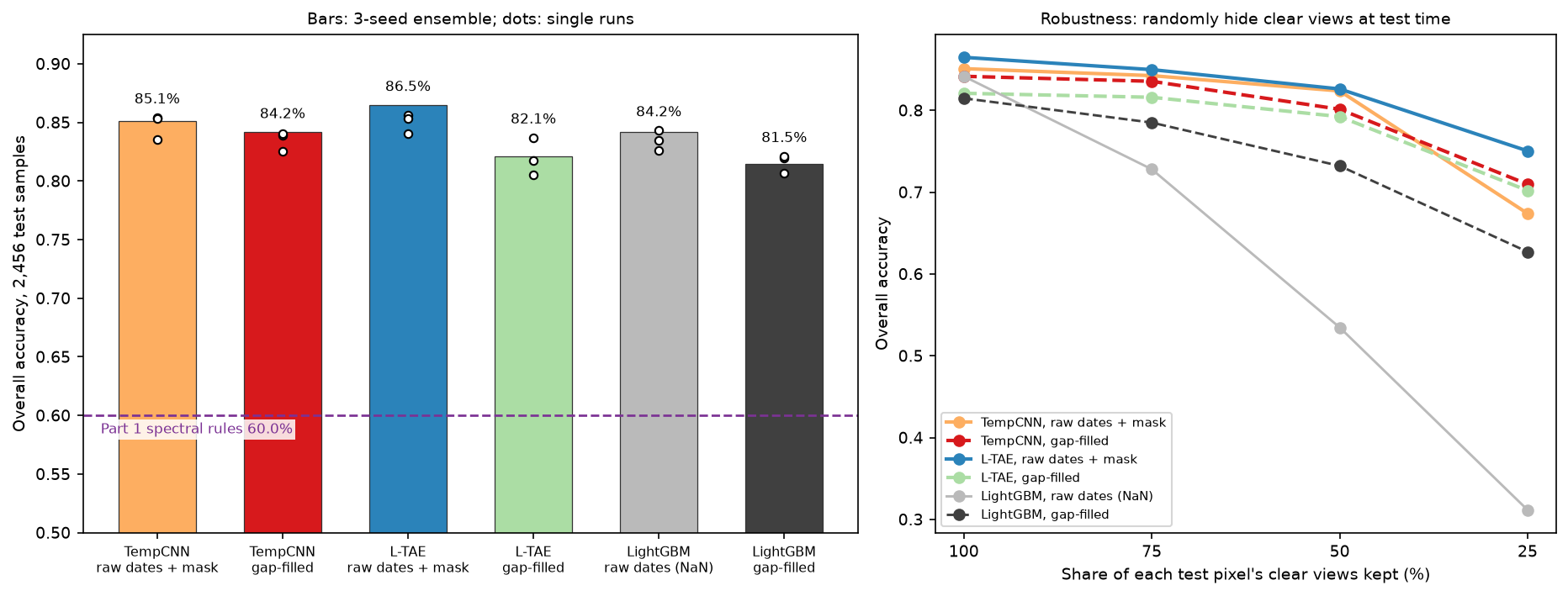
val_macro_f1 test_oa_mean test_oa_sd test_f1_mean test_f1_sd ensemble_oa ensemble_macro_f1 ensemble_kappaTempCNN, raw dates + mask 0.877 0.848 0.011 0.855 0.008 0.851 0.858 0.830TempCNN, gap-filled 0.868 0.835 0.008 0.844 0.009 0.842 0.850 0.820L-TAE, raw dates + mask 0.875 0.850 0.008 0.859 0.007 0.865 0.873 0.846L-TAE, gap-filled 0.872 0.820 0.016 0.830 0.017 0.821 0.832 0.797LightGBM, raw dates (NaN) 0.857 0.835 0.009 0.844 0.008 0.842 0.851 0.820LightGBM, gap-filled 0.840 0.816 0.008 0.826 0.007 0.815 0.826 0.790Part 1 spectral rules on the same test samples: OA 0.600, macro F1 0.630, kappa 0.547chosen on validation folds: TempCNN, raw dates + mask (deep), LightGBM, raw dates (NaN) (LightGBM)Four findings stand out.
- Every time-series model beats the Part 1 rules by more than 20 points. Using the full year, rather than three seasonal composites and eight thresholds, is the biggest single gain in this series so far.
- Masking beats gap-filling for every model: by 0.9 points for TempCNN, 4.4 for L-TAE and 2.7 for LightGBM. Linear interpolation across two-month gaps blurs exactly the timing differences the models need. The L-TAE loses most, because gap-filling removes the information it is designed to use: which dates were really observed.
- The headline model was chosen on validation, not test. TempCNN with the mask had the best mean validation F1 (0.877, against 0.875 for the L-TAE), so it is the reported model. On the test blocks, the L-TAE ensemble did better (86.5% against 85.1%). The difference is within the noise between seeds and folds, so read them as equal. If you need a model that transfers to other dates, prefer the L-TAE.
- LightGBM is close. Its best configuration reaches 84.2%.
TempCNN, raw dates + mask (3-run ensemble), n = 2,456 test samples in 27 blocksoverall accuracy 0.851 (block-bootstrap 95% CI 0.811 to 0.884); macro F1 0.858; kappa 0.830LightGBM, raw dates (NaN): OA 0.842 (95% CI 0.784 to 0.886), macro F1 0.851OA difference, deep minus LightGBM: +0.009 (paired block-bootstrap 95% CI -0.007 to +0.029)averaging the deep and LightGBM probabilities: OA 0.855, macro F1 0.863The paired block bootstrap resamples the 27 test blocks 2,000 times and recomputes the difference in accuracy on each resample. Its 95% interval, −0.7 to +2.9 points, includes zero. On 6,500 balanced training pixels, the deep model is not significantly better than gradient boosting. That is a common and useful finding: published gains for deep temporal models tend to appear with hundreds of thousands of training pixels, many more classes or transfer across years and regions. Averaging the two models’ probabilities gives a small further gain, to 85.5%, because they make partly different mistakes.
Robustness to missing dates
Another year, or another tile, will have different clouds. To simulate that, the script randomly hides 25%, 50% or 75% of each test pixel’s clear views and predicts again:
keep 100% keep 75% keep 50% keep 25%TempCNN, raw dates + mask 0.851 0.842 0.824 0.674TempCNN, gap-filled 0.842 0.836 0.801 0.710L-TAE, raw dates + mask 0.865 0.850 0.826 0.750L-TAE, gap-filled 0.821 0.816 0.792 0.702LightGBM, raw dates (NaN) 0.842 0.728 0.535 0.311LightGBM, gap-filled 0.815 0.785 0.732 0.627With half the clear views, the masked L-TAE and TempCNN still score 82%, while LightGBM on raw dates falls to 54%. Its trees split on specific dates, and when those are missing every pixel takes the same default branch. With a quarter of the views, the L-TAE keeps 75%, and the masked TempCNN drops more steeply to 67%. The comparison is not quite fair, because only the networks were trained with observation dropout. Exercise 2 below asks you to give LightGBM the same augmentation. Even so, it shows that a model which knows which dates are missing degrades gracefully.
Per-class accuracy
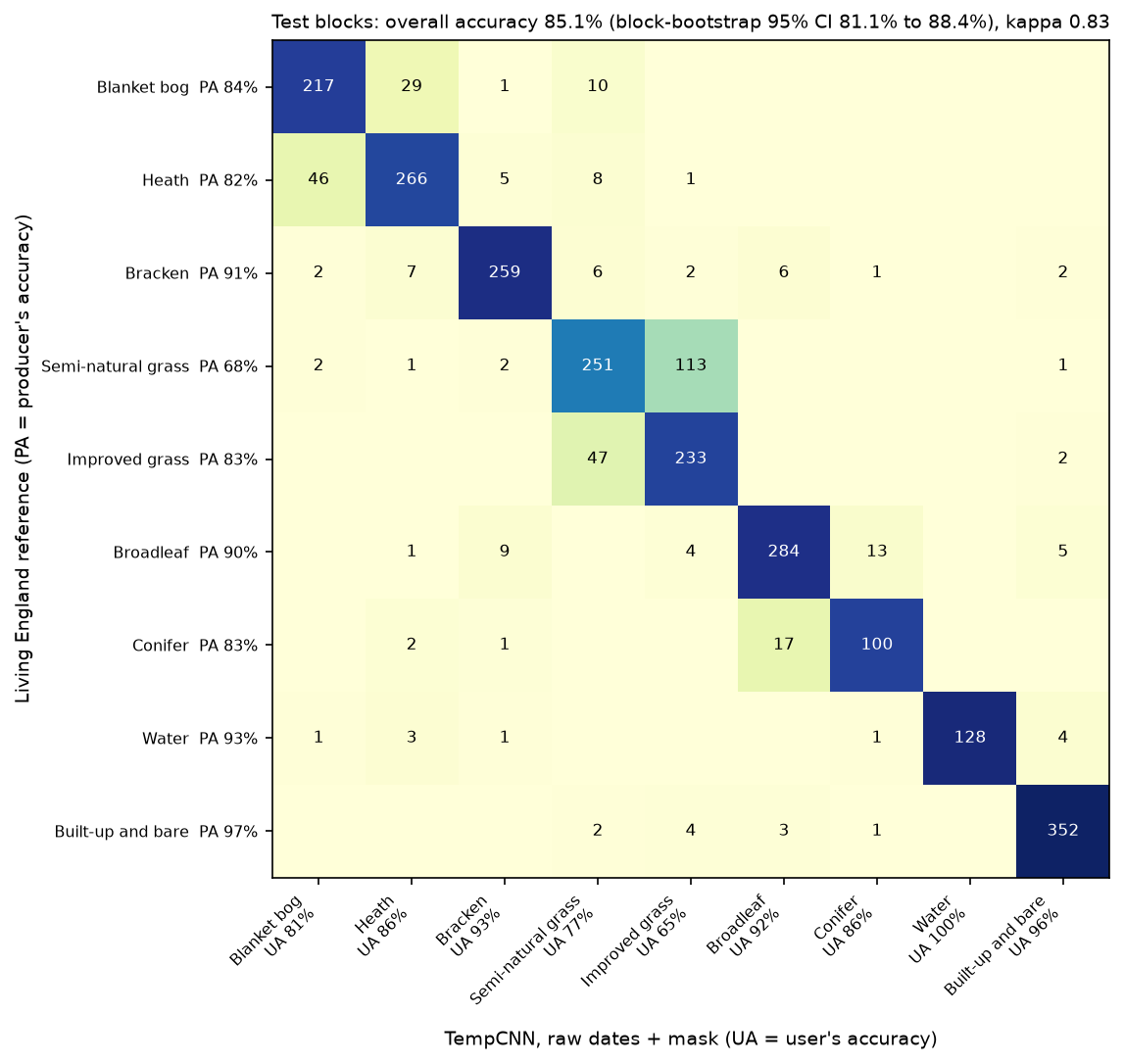
n_test producers_acc users_acc f1 f1_lightgbmBlanket bog 257 0.844 0.810 0.827 0.832Heath 326 0.816 0.861 0.838 0.835Bracken 285 0.909 0.932 0.920 0.901Semi-natural grassland 370 0.678 0.775 0.723 0.682Improved grassland 282 0.826 0.653 0.729 0.726Broadleaf woodland 316 0.899 0.916 0.907 0.911Conifer woodland 120 0.833 0.862 0.847 0.859Water 138 0.928 1.000 0.962 0.958Built-up and bare 362 0.972 0.962 0.967 0.951The two problem classes from Part 1 are transformed. Semi-natural grassland’s producer’s accuracy rises from 23% to 68%, and blanket bog’s user’s accuracy from 41% to 81%. Grassland is still the weakest class: 113 of 370 semi-natural grassland samples are called improved. Part of this is probably a label problem rather than a model problem: the line between semi-improved and unimproved pasture is hard to draw from space, and Living England draws it with a model too. Bog and heath are still confused in both directions (46 and 29 samples), which is no surprise on a moorland where the two form a fine mosaic. The deep model’s clearest gain over LightGBM is on semi-natural grassland (F1 0.72 against 0.68). LightGBM is slightly better on bog and conifer.
Step 7: which dates matter?
Attention weights
The L-TAE’s attention weights say how much each clear date contributed to each pixel’s summary. Raw weights are hard to compare, because a pixel with 10 clear dates gives each an average weight of 0.1, while one with 30 clear dates gives each 0.033. The script therefore multiplies each weight by the pixel’s number of clear dates. A value of 1 then means “an equal share”, and 2 means twice that. These relative weights are averaged over the test pixels, the three seeds and the 16 heads.
top 6 dates: 04 Apr 1.61, 22 Mar 1.35, 24 May 1.33, 03 Sep 1.28, 07 Mar 1.26, 25 Nov 1.21bottom 3 dates: 22 Aug 0.50, 03 Oct 0.47, 16 May 0.47 Blanket bog most attended date 24 May (1.92) Bracken most attended date 03 Sep (2.28) Semi-natural grassland most attended date 04 Apr (2.00) Improved grassland most attended date 04 Apr (2.27) Broadleaf woodland most attended date 03 Sep (1.54)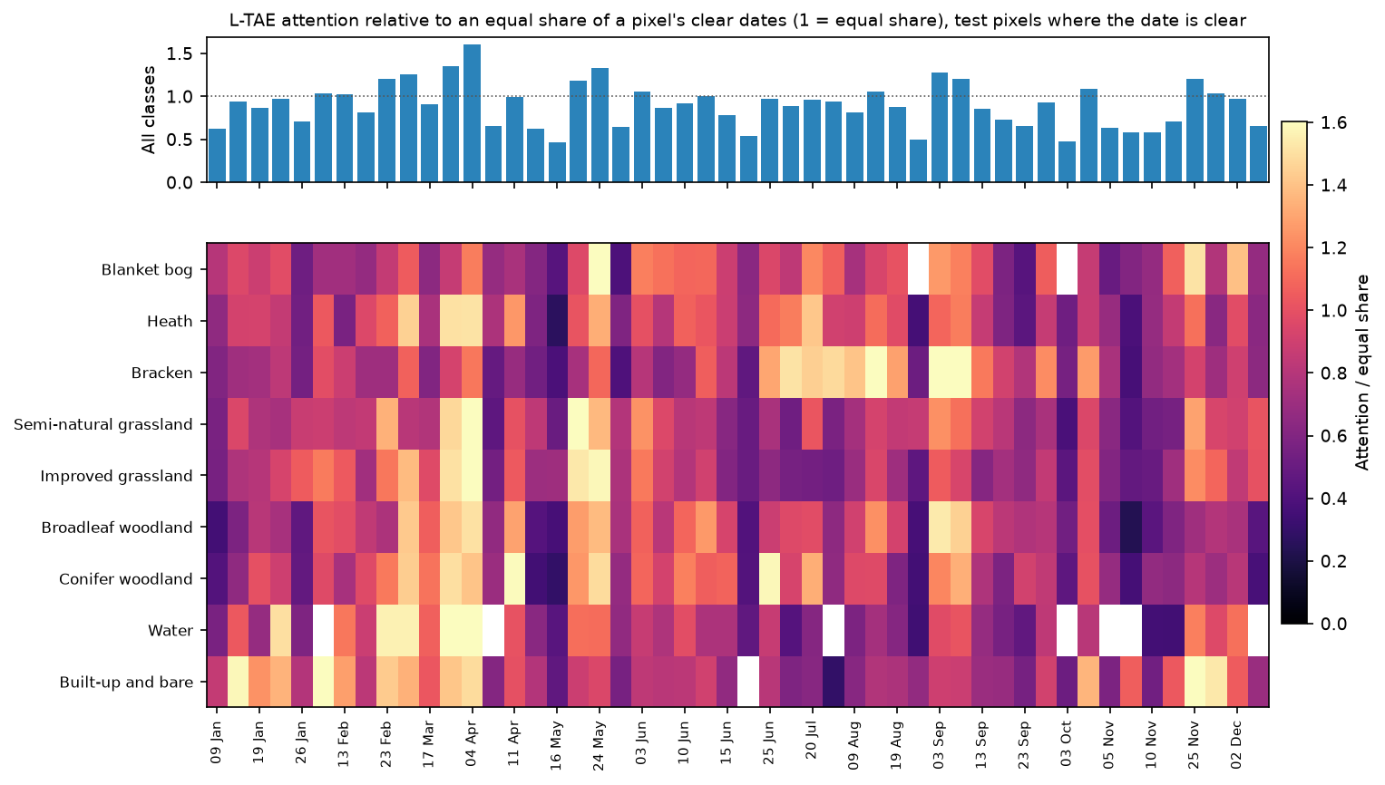
The patterns make ecological sense. Early April, before the grasses green up, is when improved grassland already looks green and semi-natural grassland and heather still look brown. Bracken is recognised from late June to early September, when its dense canopy is fully out. Woodland draws on spring, before and after leaf-out, and on early September. Built-up land uses winter dates, when bare ground and roofs stand out most against dormant vegetation.
Two warnings apply. Attention shows where the model looked, not what caused its decision, and the two can differ (Jain and Wallace 2019). And a date can score low because it is redundant with a neighbouring date, not because it is useless.
Occlusion by month
A more direct test is to take information away. The script hides every clear view in one month at a time, as if the whole month had been cloudy, and measures the drop in test accuracy:
for mo in range(1, 13): mo_mask = mt & (dates.month.to_numpy() != mo)[None, :] # pretend every view in this month was cloudy drops.append(base - (ens_proba(cfg, XN[te], mo_mask).argmax(1) == yt).mean()) Jan Feb Mar Apr May Jun Jul Aug Sep Oct Nov DecL-TAE, raw dates + mask -0.4 0.6 -0.4 0.4 1.1 4.2 -0.1 0.2 0.9 -0.3 0.2 0.4TempCNN, gap-filled -1.3 -0.3 0.3 0.7 1.8 2.2 -0.0 0.2 0.9 0.4 0.4 0.9LightGBM, raw dates (NaN) -0.1 -0.0 -0.3 10.2 8.1 13.7 0.0 0.2 4.3 0.2 1.1 1.4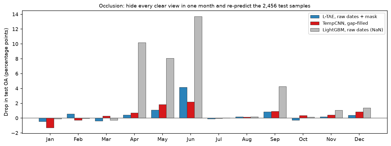
For the networks, no single month is critical. June, the clearest month with 69% of observations clear, costs the L-TAE 4.2 points, and no other month costs more than 2. Small negative values (hiding January helps by up to 1.3 points) are noise, and a hint that winter views add little. The occlusion and attention results agree on spring and early September. They differ on June, which gets ordinary attention per date but holds many of the year’s clear views, so removing it removes a lot of data at once. LightGBM’s dependence on April to June is again striking. It is the same weakness that the robustness test exposed.
Step 8: a wall-to-wall map on a CPU
Predicting the whole 25 × 22.5 km area needs every band on every date for every pixel: 50 dates × 10 bands × 5.6 million pixels. As 16-bit integers that is 5.6 GB, too much for many laptops’ memory but fine on disk. The script downloads each date once, writes it into a memory-mapped NumPy file, then reads it back in strips of 50 rows (about 250 MB each as 32-bit floats). Only one strip is in memory at a time, so full 10 m resolution is feasible on a 16 GB laptop, and there is no need to fall back to a subset or a coarser grid. Disk space is the real cost. The download took about 4 minutes and the prediction 7 minutes on 8 threads.
mm = np.lib.format.open_memmap(STACK, mode="w+", dtype="int16", shape=(T, C, R, W))for i, t in enumerate(dates):                                  # one date at a time: low memory    day = ds.sel(time=t).compute()    for b, band in enumerate(BANDS):        mm[i, b] = np.clip(day[band].values.astype("int32") - off[t], -32768, 32767).astype("int16")
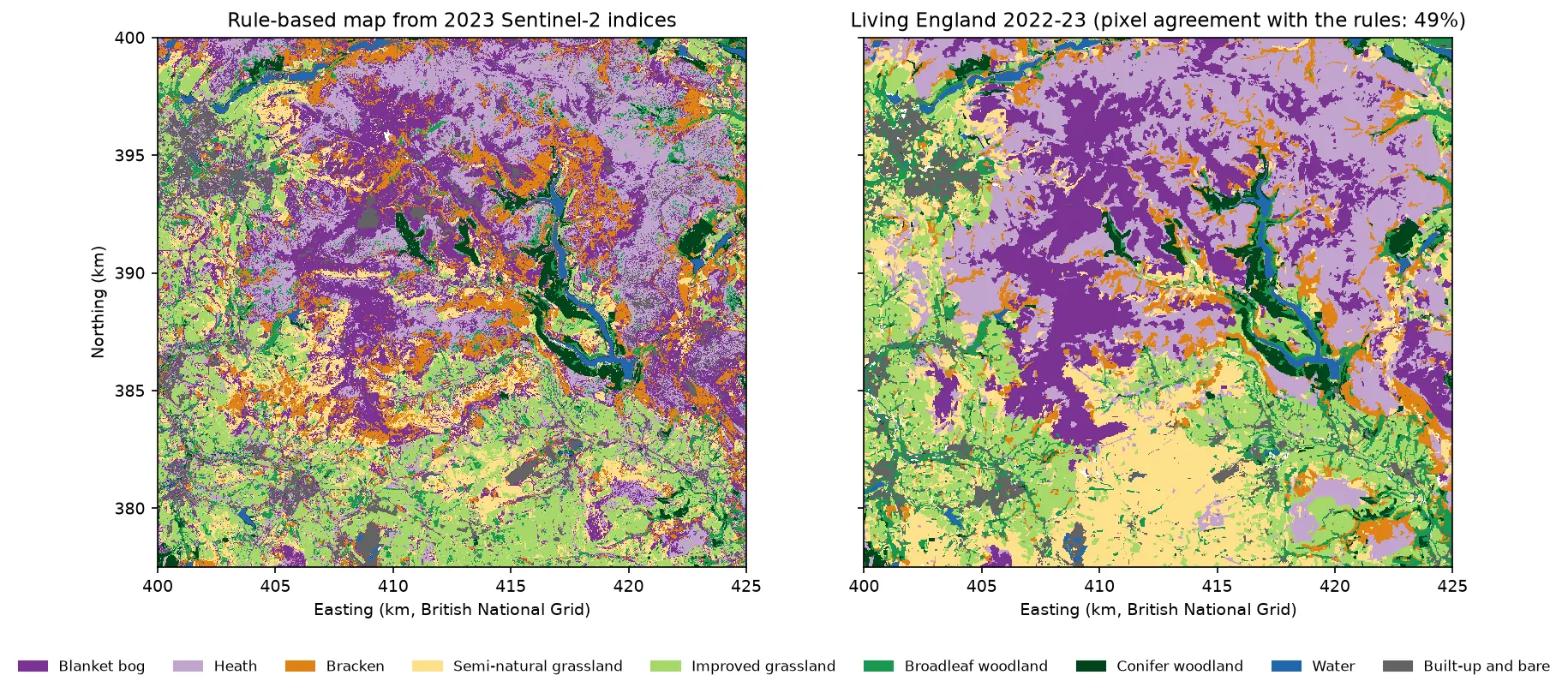
stack = np.load(STACK, mmap_mode="r")for r0 in range(0, R, STRIP): # strips of 50 rows x 2,500 columns r1 = min(R, r0 + STRIP) xs = np.asarray(stack[:, :, r0:r1, :], dtype="float32") / 10000 xs = xs.transpose(2, 3, 0, 1).reshape(-1, T, C) # (pixels, dates, bands) ms = clear[:, r0:r1, :].transpose(1, 2, 0).reshape(-1, T) xn = np.where(ms[..., None], (xs - mu) / sd, 0.0).astype("float32") p = ens_proba(BEST, xn, ms) # average of the three runs pred[r0:r1] = (p.argmax(1) + 1).reshape(r1 - r0, W)downloaded the 50-date x 10-band stack in 250 sstack: (50, 10, 2250, 2500) int16 on disk = 5.6 GB (memory-mapped, read in strips)predicted 5,625,000 pixels with TempCNN, raw dates + mask (3-run ensemble) in 427 s; 0.000% never clearwall-to-wall agreement with Living England: test blocks 0.699, whole study area 0.717 (Part 1 rules: 0.483 and 0.490) model_km2 living_england_km2Blanket bog 94.9 90.5Heath 115.8 151.5Bracken 46.6 41.6Semi-natural grassland 109.9 96.1Improved grassland 88.5 90.0Broadleaf woodland 45.2 39.7Conifer woodland 16.4 17.2Water 8.0 8.4Built-up and bare 37.2 25.7median top-class probability 0.87; 7.6% of pixels below 0.5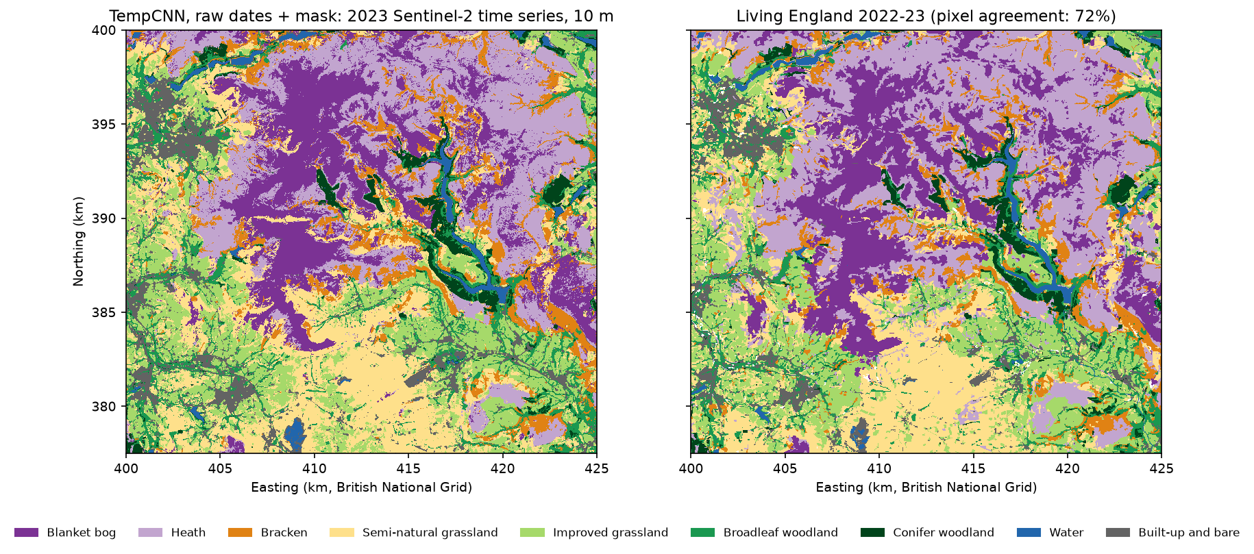
Every pixel had at least one clear view in 2023, so the whole area is mapped. The map agrees with Living England on 70% of the test blocks and 72% of the whole area, against 48% and 49% for the Part 1 rules. Those figures are lower than the 85% sample accuracy because the samples are pure pixels in reliable polygons, whereas the map includes edges, mixed pixels and Living England’s own errors.
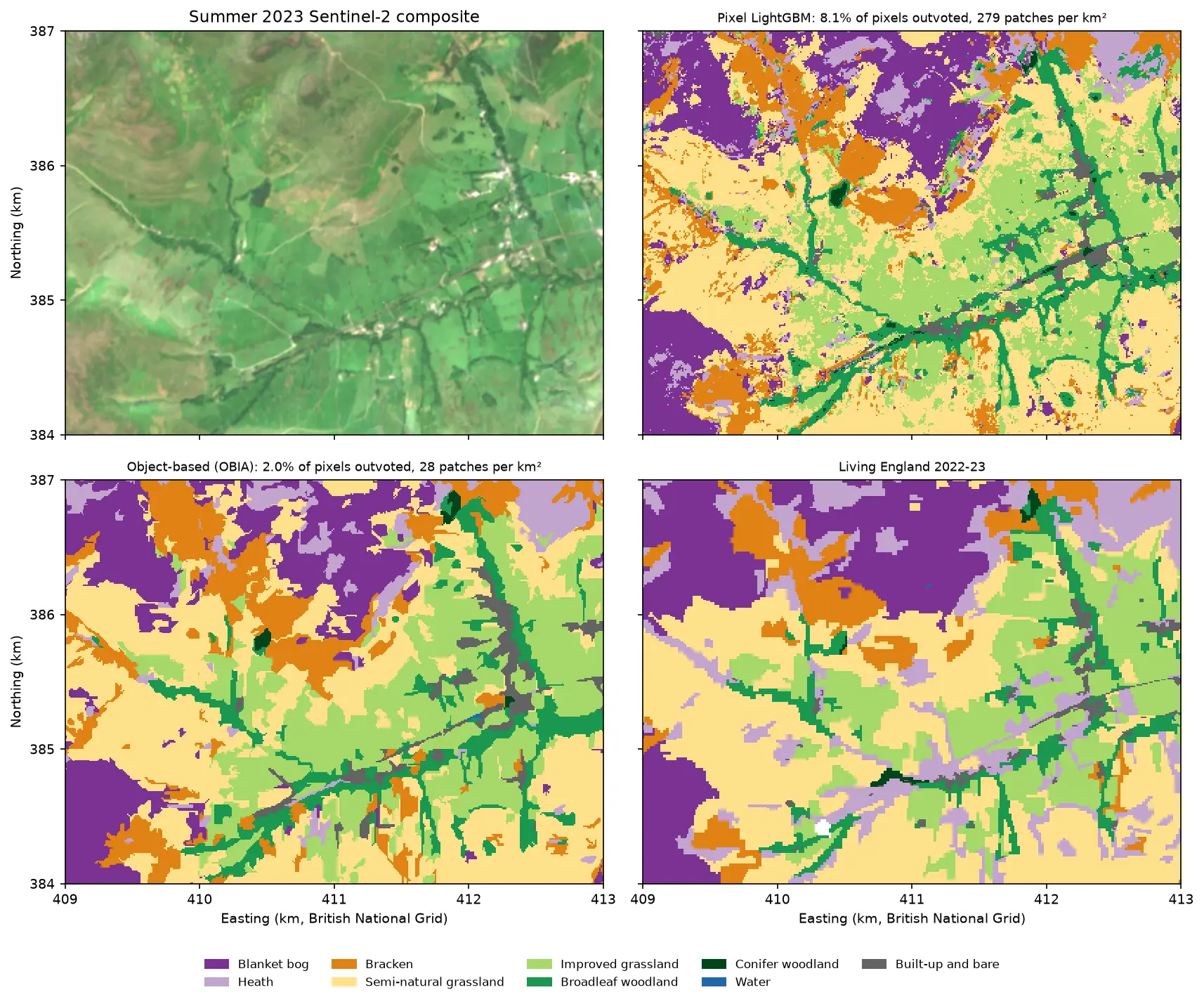
The area table shows the model’s biases. It maps 36 km² less heath than Living England, and more bog, bracken and semi-natural grassland. It also maps 11 km² more built-up and bare land, probably including eroded peat on the plateaux, which Living England often folds into the surrounding bog. Pixel classifiers also leave fine speckle along habitat boundaries. Part 3’s object-based approach is one answer to that.
Comparison with the Part 1 baseline
| Measure (test blocks, n = 2,456) | Part 1: spectral rules | LightGBM, raw dates | TempCNN, raw dates + mask | L-TAE, raw dates + mask |
|---|---|---|---|---|
| Overall accuracy | 0.600 (CI 0.527 to 0.664) | 0.842 (CI 0.784 to 0.886) | 0.851 (CI 0.811 to 0.884) | 0.865 |
| Macro F1 | 0.630 | 0.851 | 0.858 | 0.873 |
| Cohen’s kappa | 0.547 | 0.820 | 0.830 | 0.846 |
| Semi-natural grassland PA | 0.227 | 0.678 | ||
| Blanket bog UA | 0.407 | 0.810 | ||
| Wall-to-wall agreement, test blocks | 0.483 | 0.699 | ||
| Wall-to-wall agreement, whole area | 0.490 | 0.717 | ||
| Training-block validation | OA 0.684 ± 0.030 (5-fold blocked CV) | macro F1 0.857 (3 spatial folds) | macro F1 0.877 | macro F1 0.875 |
All confidence intervals are block-bootstrap 95% intervals. The validation row is not directly comparable across columns: Part 1 used blocked 5-fold CV of overall accuracy, while this part reports the mean macro F1 on three held-out spatial folds.
Limitations
- The labels are a model. Living England is itself a classification of Sentinel-1 and Sentinel-2 data, with its own errors. A model that learns to reproduce it can score highly by copying those errors, and its “mistakes” may sometimes be right.
- Balanced, pure samples flatter accuracy. The test samples are 1,000 per class from the interiors of reliable polygons. The 85% is sample accuracy, not map accuracy; the 70% wall-to-wall agreement is closer to what a user of the map would see. Part 5 covers area-weighted accuracy.
- One tile, one year. All pixels share the same 50 acquisition dates in 2023, so TempCNN can learn “position 12 means 4 April”. A different year, or a pixel in a neighbouring tile, breaks that assumption. The L-TAE’s day-of-year encoding should transfer better, but this tutorial does not test it.
- A confounded robustness test. The networks were trained with observation dropout and LightGBM was not, so the robustness comparison favours the networks.
- Small differences between deep models. Seeds and folds move accuracy by about 1 point, which is as large as the gaps between TempCNN, L-TAE and LightGBM with masked inputs. Three seeds are the minimum for an honest comparison; more would be better.
- Clouds the mask misses. The clear flag comes from the Sentinel-2 scene classification layer, which misses some thin cloud, shadow and snow. These leak into the “clear” views as noise.
Try it yourself
- Remove the augmentation. Set
P_DROP = 0and rerun. How much of the networks’ advantage in the robustness test disappears? - Give LightGBM the same augmentation. Stack three copies of the training rows, each with a random 20% of clear views set to NaN. Does its collapse at 50% of views go away?
- Shift the calendar. Add 30 days to
DOYat test time only and predict with the L-TAE. A large drop shows that the model relies on the date, not just the order of observations. - Swap in a Transformer. Replace the L-TAE with
nn.TransformerEncoder(two layers, four heads, a learned class token) using the samedoy_encoding. Compare its accuracy, parameter count and training time. - Coarser gap-filling. Change
GRIDto a 5-day or 20-day step. Does a finer grid narrow the gap between gap-filling and masking? - Map the uncertainty. Save
confas a GeoTIFF and overlay it on the map. Are the low-confidence pixels on the bog–heath mosaic and the limestone grasslands?
Frequently asked questions
What is the best deep learning model for satellite image time series classification?
There is no single best model, but two families are reliable starting points. A 1D convolutional network such as TempCNN is simple, fast and hard to beat when all pixels share the same dates. Attention models such as L-TAE or a small Transformer encoder with a day-of-year encoding handle irregular, cloudy dates directly and transfer better to new dates. In this tutorial they were within about 1 point of each other. Recurrent networks (LSTM, GRU) also work but are slower to train and rarely better.
Do I need to gap-fill cloudy Sentinel-2 time series before deep learning?
No, and here it hurt. Feeding the raw dates with a clear-sky mask beat linear gap-filling onto a 10-day grid for every model, by 0.9 to 4.4 points of overall accuracy. Gap-filling is still useful when a model needs a fixed, regular input, such as a CNN applied to data from different tiles or years. If you gap-fill, keep the grid fine and consider passing the number of days to the nearest real observation as an extra channel.
Is deep learning better than random forest or LightGBM for time series classification?
Not necessarily. On 6,500 training pixels, LightGBM on the same per-date values was within 1 point of the best deep model, and the difference was not significant. Deep temporal models tend to pull ahead with much larger training sets, many classes, or when the model must cope with different dates and missing data. That last point was the networks’ clearest advantage here. Always train a strong tree-based baseline on the same inputs before claiming a deep-learning gain.
Can I train a deep learning model on satellite time series without a GPU?
Yes. Pixel-level temporal models are small: the L-TAE here has 44,000 parameters and trains in under a minute on 8 CPU threads, and TempCNN in about a minute. All 18 models in this tutorial trained in 8 minutes. Wall-to-wall prediction of 5.6 million pixels took 7 minutes. Spatio-temporal models that process image patches through time, such as U-TAE, are much heavier and do benefit from a GPU.
What is the difference between L-TAE and a Transformer?
L-TAE is a stripped-down Transformer encoder for time series classification. A Transformer computes a query for every input date and T × T attention weights, then stacks several layers. L-TAE learns one “master” query per attention head, pools the whole sequence in a single step, and gives each head its own group of channels. The result is far fewer parameters and one interpretable weight per date, with accuracy similar to a full Transformer on tasks like this one.
How do I know which dates matter to the model?
Use two complementary tools. Attention weights, from models that have them, show where the model looked. Occlusion, which hides a date or a month and measures the drop in accuracy, shows what the model actually needs. In this tutorial attention peaked in early April, late May and early September, and hiding June cost the most accuracy. Attention is cheap but is not a causal explanation; occlusion is slower but more direct.
Next steps
- Go back to Part 1: habitat mapping with Sentinel-2 in Python for the study area, the labels and the accuracy assessment that this part builds on.
- See whether a foundation model can match the deep models with a fraction of the labels in Part 5: AlphaEarth satellite embeddings in Python, which also compares all five methods in the series.
- Learn more about loading Sentinel-2 time series from STAC in NDVI time series with odc-stac, and improve the clear-sky mask with Sentinel-2 cloud masking in Python.
- For a spatial model rather than a temporal one, train a U-Net for satellite image segmentation, and see deep learning inference on large rasters for tiling and memory tricks.
- Add radar to the time series with Sentinel-1 crop monitoring: per-date VV and VH backscatter are cloud-free extra channels for the same models.
Data and licences
- Living England Habitat Map 2022-23: © Natural England, under the Open Government Licence v3.0. Contains Ordnance Survey data © Crown copyright and database right. Accessed from Natural England’s public ArcGIS service on 21 October 2026.
- Sentinel-2 L2A: contains modified Copernicus Sentinel data 2023, free and open under the Copernicus data licence. Accessed from the Microsoft Planetary Computer.
- References: Pelletier, C., Webb, G. I. and Petitjean, F. (2019), “Temporal convolutional neural network for the classification of satellite image time series”, Remote Sensing 11(5), 523. Garnot, V. S. F. and Landrieu, L. (2020), “Lightweight temporal self-attention for classifying satellite images time series”, in Advanced Analytics and Learning on Temporal Data (AALTD 2020), Springer LNCS 12588. Garnot, V. S. F. and Landrieu, L. (2021), “Panoptic segmentation of satellite image time series with convolutional temporal attention networks”, ICCV 2021. Vaswani, A. et al. (2017), “Attention is all you need”, NeurIPS 2017. Rußwurm, M. and Körner, M. (2020), “Self-attention for raw optical satellite time series classification”, ISPRS Journal of Photogrammetry and Remote Sensing 169, 421–435. Jain, S. and Wallace, B. C. (2019), “Attention is not explanation”, NAACL 2019.
- Code:
habitat_time_series_dl.pyand the shared series module (habitat_common.py,prepare_data.py, sample CSVs), tested with Python 3.12.0, PyTorch 2.14.1 (CPU), LightGBM 4.7.0, NumPy 2.5.4, pandas 3.0.6, odc-stac 0.5.3 and matplotlib 3.11.2.
Key terms
- Satellite image time series (SITS)
- A stack of images of the same place at many dates. For classification, each pixel becomes a sequence of spectra, so the model can use how a surface changes through the year, not just how it looks on one day.
- TempCNN
- A temporal convolutional neural network (Pelletier et al. 2019) that slides one-dimensional filters along the time axis of a pixel's time series, much as an image CNN slides two-dimensional filters across space.
- Attention
- A learned weighted average. The model scores every input element, here every date, turns the scores into weights that sum to one with a softmax, and averages the inputs with those weights.
- Positional encoding
- Extra numbers added to each input element to tell an attention model where it sits in the sequence. Attention itself ignores order, so for time series the encoding carries the date.
- L-TAE
- The Lightweight Temporal Attention Encoder (Garnot and Landrieu 2020). A slimmed-down Transformer encoder for satellite time series that uses one learned query per attention head and splits the channels between heads.
- Gap-filling
- Replacing cloudy or missing observations with estimates, here by linear interpolation between the nearest clear views, usually onto a regular time grid.
Data for this tutorial
- Living England Habitat Map · Natural England's broad habitat map, used as labels (2022-23 release)
- Microsoft Planetary Computer · Sentinel-2 L2A through STAC, no account needed
Licences and formats for each source are listed in the GIS data sources catalogue.