U-Net satellite image segmentation in PyTorch: a TorchGeo and Sentinel-2 tutorial on a CPU

Short answer: to train a U-Net for satellite image segmentation in PyTorch, load your image chips and masks into a Dataset and build the model with segmentation_models_pytorch: smp.Unet("resnet18", in_channels=13, classes=5). Load a Sentinel-2 pretrained encoder from TorchGeo (ResNet18_Weights.SENTINEL2_ALL_MOCO) into model.encoder. Train with AdamW on a weighted cross-entropy plus Dice loss, with flips and rotations as augmentation. Then score it on spatially separate test chips with per-class IoU, F1 and a confusion matrix. A small U-Net on 128-pixel chips trains in minutes on a CPU.

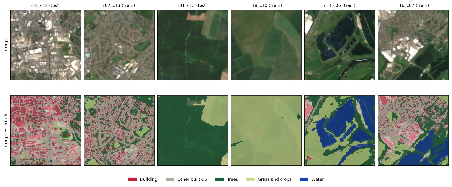
This is part 2 of the series Deep learning for satellite imagery with Python. Part 1 built 576 labelled Sentinel-2 chips of Nottingham, with five classes from Overture building footprints and ESA WorldCover 2021, split into training, validation and test sets by 5 km blocks. Here we train a U-Net on them, on an ordinary CPU, and look closely at what it gets right and wrong. Part 3 runs the trained model over a whole new city.

You will learn how to:

1. load georeferenced image chips into a PyTorch Dataset, with augmentation;
2. build a U-Net with segmentation_models_pytorch and load TorchGeo’s Sentinel-2 pretrained weights into its encoder;
3. handle class imbalance with a weighted cross-entropy plus Dice loss;
4. train on a CPU in about five minutes, and plot real loss curves;
5. report IoU, F1 and a confusion matrix per class, and compare pretrained weights, random weights and a leaky random split.

All outputs below come from train_unet.py, run on 19 October 2026 with Python 3.12, PyTorch 2.14.1 (CPU), segmentation-models-pytorch 0.5.0 and TorchGeo 0.10.1. The machine was a desktop AMD Ryzen 9 7950X, limited to 8 threads, with no GPU. The script trains three models and took about 16 minutes in total.

Install PyTorch for CPU

Install the CPU build of PyTorch first from PyTorch’s own index; on Linux, the default wheels include CUDA and weigh several gigabytes. Then install the rest:

python -m venv .venv-dl
.venv-dl\Scripts\activate          # on macOS or Linux: source .venv-dl/bin/activate
pip install torch==2.14.1 torchvision==0.29.1 --index-url https://download.pytorch.org/whl/cpu
pip install -r requirements.txt    # torchgeo, segmentation-models-pytorch, rasterio, geopandas, ...

Step 1: get the chips from part 1

The script expects part 1’s chips in the folder next to it: ../satellite-imagery-training-data-python/data/chips/. If you skipped part 1, you do not need to do anything. If the chips are missing, the script downloads make_training_chips.py from this site and runs it first. That streams the Sentinel-2 imagery and Overture buildings and takes a few minutes. If your chips are somewhere else, set the CHIPS_DIR environment variable.

PART1 = HERE.parent / "satellite-imagery-training-data-python"
CHIPS = Path(os.environ.get("CHIPS_DIR", PART1 / "data" / "chips"))
if not (CHIPS / "chips.gpkg").exists():
    script = PART1 / "make_training_chips.py"
    if not script.exists():                       # skipped part 1: fetch its script from the site
        PART1.mkdir(parents=True, exist_ok=True)
        url = os.environ.get("TGIS_CODE_URL", "https://www.technicalgis.com/code")
        urllib.request.urlretrieve(f"{url}/satellite-imagery-training-data-python/make_training_chips.py", script)
    subprocess.run([sys.executable, str(script)], check=True, cwd=PART1)

chips = gpd.read_file(CHIPS / "chips.gpkg")
X, Y = map(np.stack, zip(*(read(c) for c in chips["chip_id"])))

All 576 chips fit comfortably in memory (226 MB as uint16), so we read them once:

loaded 576 chips in 4.8 s: X (576, 12, 128, 128) uint16, Y (576, 128, 128) uint8
bands: B01, B02, B03, B04, B05, B06, B07, B08, B8A, B09, B11, B12
split
train    416
val       80
test      80

Step 2: a Dataset that matches the pretrained encoder

A pretrained encoder only helps if you feed it data the way it was trained. TorchGeo’s Sentinel-2 ResNet-18 weights were trained on all 13 bands of Sentinel-2 L1C data, divided by 10,000. Our chips are L2A, which has 12 bands because B10, the cirrus band, is dropped. So we scale the reflectance the same way and insert a channel of zeros where B10 would be.

Augmentation matters with only 416 training chips. Satellite images have no “up”, so all eight flips and rotations of a square are valid. We apply the same transform to the image and to the mask:

def to_input(x: np.ndarray) -> torch.Tensor:
    x = torch.from_numpy(x.astype("float32") / 10000)
    return torch.cat([x[..., :10, :, :], torch.zeros_like(x[..., :1, :, :]), x[..., 10:, :, :]], dim=-3)


class ChipDataset(Dataset):
    def __init__(self, idx: np.ndarray, augment: bool = False):
        self.idx, self.augment = idx, augment

    def __len__(self):
        return len(self.idx)

    def __getitem__(self, i):
        x, y = to_input(X[self.idx[i]]), torch.from_numpy(Y[self.idx[i]].astype("int64"))
        if self.augment:                                  # the 8 flips and rotations of a square
            k = int(torch.randint(4, (1,)))
            x, y = torch.rot90(x, k, (1, 2)), torch.rot90(y, k, (0, 1))
            if torch.rand(1) < 0.5:
                x, y = x.flip(2), y.flip(1)
        return x, y

Step 3: a U-Net with a Sentinel-2 pretrained encoder

segmentation_models_pytorch (smp) builds a U-Net around any of dozens of encoders in one line. Its built-in pretrained weights come from ImageNet photographs with three bands. TorchGeo provides weights trained on Sentinel-2 itself. SENTINEL2_ALL_MOCO is a ResNet-18 pretrained on the SSL4EO-S12 dataset with MoCo, a self-supervised method that needs no labels.

Both libraries use the same ResNet-18 layer names, so we can drop TorchGeo’s classifier layer (fc) and load the rest straight into smp’s encoder:

WEIGHTS = ResNet18_Weights.SENTINEL2_ALL_MOCO


def make_model(pretrained: bool, quiet: bool = True) -> torch.nn.Module:
    torch.manual_seed(SEED)
    model = smp.Unet("resnet18", encoder_weights=None, in_channels=13, classes=NC)
    if pretrained:
        sd = {k: v for k, v in WEIGHTS.get_state_dict(progress=False).items() if not k.startswith("fc.")}
        torch.nn.Module.load_state_dict(model.encoder, sd, strict=True)    # strict: every tensor must match
    return model

loaded SENTINEL2_ALL_MOCO into the encoder: 120 tensors, classifier head dropped
U-Net, ResNet-18 encoder: 14.4 M parameters (11.2 M in the encoder)

ResNet-18 is a modest encoder by today’s standards, which is the point here: it trains on a CPU. TorchGeo also has Sentinel-2 weights for ResNet-50 and ViT encoders, which are worth trying if you have a GPU.

Step 4: loss, metrics and the training loop

Part 1 showed that grass and crops cover 60% of the labelled pixels and water just 1.3%. We weight the cross-entropy loss by the inverse square root of each class’s frequency, and add a Dice loss, which scores each class’s overlap separately and so does not let the big classes dominate. Pixels labelled 255 are ignored by both.

counts = np.bincount(Y[(chips["split"] == "train").to_numpy()].ravel(), minlength=256)[:NC]
class_w = torch.tensor(1 / np.sqrt(counts / counts.sum()), dtype=torch.float32)
class_w /= class_w.mean()
dice = smp.losses.DiceLoss("multiclass", ignore_index=IGNORE)


def loss_fn(logits, y):
    return F.cross_entropy(logits, y, weight=class_w, ignore_index=IGNORE) + dice(logits, y)

The metrics all come from one pixel confusion matrix, accumulated over the validation or test chips. Computing IoU per chip and then averaging would give too much weight to chips where a class covers a handful of pixels.

def scores(cm: np.ndarray) -> pd.DataFrame:
    tp = np.diag(cm)
    fp, fn = cm.sum(0) - tp, cm.sum(1) - tp
    return pd.DataFrame({"IoU": tp / (tp + fp + fn), "F1": 2 * tp / (2 * tp + fp + fn),
                         "precision": tp / (tp + fp), "recall": tp / (tp + fn),
                         "share": cm.sum(1) / cm.sum()}, index=CLASSES)

The training loop is plain PyTorch, with no framework. AdamW with a one-cycle learning rate schedule converges reliably in a few epochs. After each epoch, we score the validation chips and keep the weights from the epoch with the best validation mean IoU:

EPOCHS, BATCH, LR = 30, 16, 1e-3
...
    opt = torch.optim.AdamW(model.parameters(), lr=LR, weight_decay=1e-4)
    sched = torch.optim.lr_scheduler.OneCycleLR(opt, max_lr=LR, total_steps=EPOCHS * len(train_dl), pct_start=0.15)
    for epoch in range(1, EPOCHS + 1):
        model.train()
        for x, y in train_dl:
            opt.zero_grad()
            loss = loss_fn(model(x), y)
            loss.backward()
            opt.step()
            sched.step()
        cm, vl = confusion(model, val_dl)
        miou = scores(cm)["IoU"].mean()
        if miou > best:
            best, state = miou, {k: v.clone() for k, v in model.state_dict().items()}

We train three models with exactly the same settings and seed: the pretrained encoder on the block split, the same network from random weights, and the pretrained encoder on a random chip split, the leaky kind that part 1 warned about.

=== training: 30 epochs, batch 16, AdamW + one-cycle, weighted cross-entropy + Dice ===
class weights: Building 1.27, Other built-up 0.71, Trees 0.53, Grass and crops 0.32, Water 2.17
pretrained encoder     epoch  1: train loss 2.922 | val loss 2.599 | val mIoU 0.090 | 0.1 min
pretrained encoder     epoch  2: train loss 2.248 | val loss 2.326 | val mIoU 0.243 | 0.3 min
pretrained encoder     epoch  5: train loss 1.128 | val loss 2.197 | val mIoU 0.323 | 0.7 min
pretrained encoder     epoch 10: train loss 0.874 | val loss 0.932 | val mIoU 0.564 | 1.5 min
pretrained encoder     epoch 15: train loss 0.872 | val loss 0.992 | val mIoU 0.547 | 2.2 min
pretrained encoder     epoch 20: train loss 0.803 | val loss 0.839 | val mIoU 0.611 | 3.1 min
pretrained encoder     epoch 25: train loss 0.771 | val loss 0.800 | val mIoU 0.622 | 3.9 min
pretrained encoder     epoch 30: train loss 0.766 | val loss 0.799 | val mIoU 0.622 | 4.8 min
pretrained encoder: 416 training chips, 4.8 min; best val mIoU 0.623 at epoch 29
from scratch: 416 training chips, 4.9 min; best val mIoU 0.619 at epoch 28
random split (leaky): 386 training chips, 5.5 min; best val mIoU 0.633 at epoch 30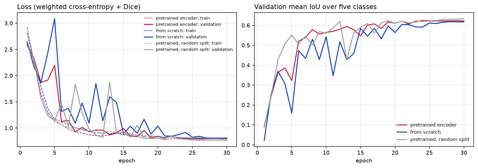

The training and validation losses end close together (0.766 and 0.799), so the model is not badly overfitting. With 416 chips and heavy augmentation, it is more likely to be underfitting. More epochs and a bigger encoder would probably help a little, but Step 6 shows that the labels limit it more than the network does.

Step 5: test on blocks the model never saw

The test set is 80 chips in five 5 km blocks that the model never saw during training or model selection. These are the only numbers worth reporting:

=== test set: 80 chips in 5 km blocks never seen in training (1.31 M pixels) ===
                   IoU     F1  precision  recall  share
Building         0.210  0.347      0.427   0.293  0.040
Other built-up   0.581  0.735      0.672   0.811  0.123
Trees            0.711  0.831      0.819   0.843  0.260
Grass and crops  0.878  0.935      0.954   0.917  0.562
Water            0.837  0.911      0.874   0.952  0.015

                          overall accuracy  mean IoU  macro F1  Building IoU
pretrained, block split              0.860     0.643     0.752         0.210
scratch, block split                 0.858     0.638     0.745         0.190
pretrained, random split             0.851     0.616     0.730         0.182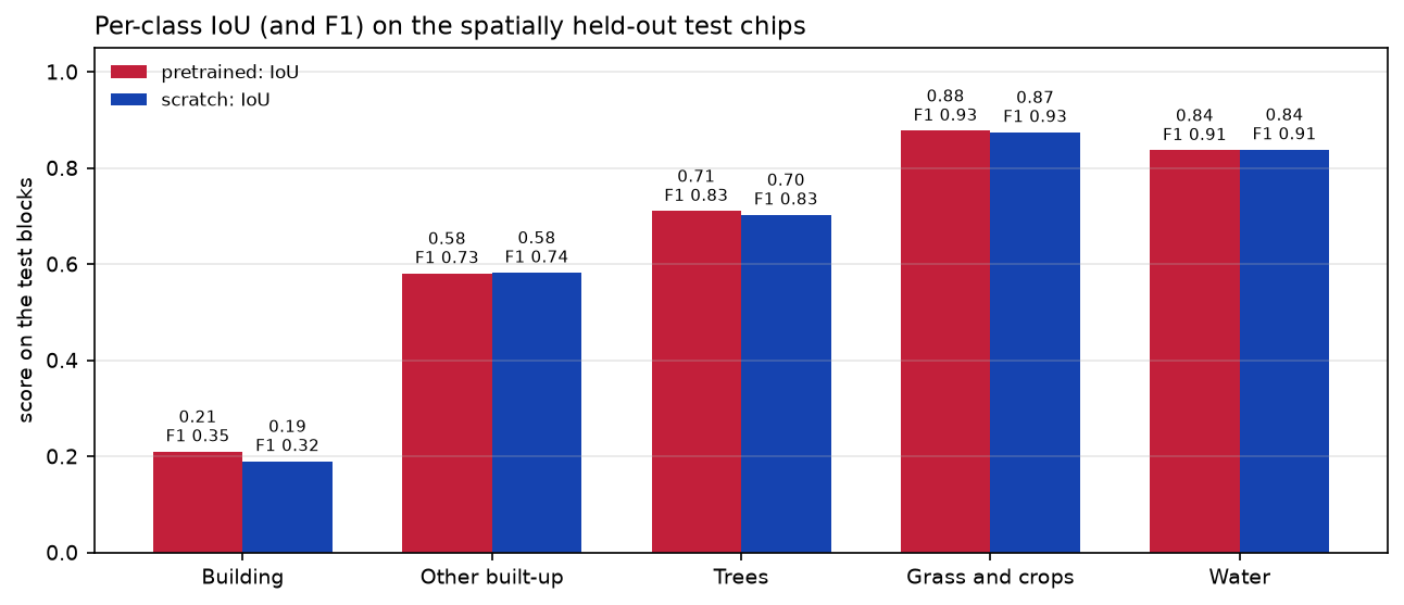

Three results stand out.

• Water, grass and crops, and trees are good. IoUs of 0.84, 0.88 and 0.71 are respectable for a five-minute CPU model trained on one city. Water has the highest recall (95%), even though it is only 1.5% of the test pixels: the class weights did their job.
• Pretraining helped training more than the result. The pretrained encoder trained more smoothly, but it beat random weights by only 0.005 mean IoU and 0.02 building IoU on the test set. The SSL4EO weights were learned from L1C top-of-atmosphere data with 13 bands, and we feed them L2A with a blank B10. With more varied training data, or fewer training chips, the gap is usually larger.
• The random split did not flatter the score here. We expected the leaky random split to report a higher score. Its validation mean IoU was indeed the highest (0.633), but its own random test chips scored 0.616. The two test sets contain different chips, so the scores are not directly comparable, and at 10 m with smooth WorldCover labels there is little fine detail to memorise. The block split is still the right choice. It is the only one whose test score is a fair estimate for a new area, and part 3 checks that estimate on a different city.

Step 6: the confusion matrix, and what limits accuracy

Per-class scores tell you which class is weak; the confusion matrix tells you why:

                 Building  Other built-up  Trees  Grass and crops  Water
Building             29.3            61.1    7.9              1.7    0.0
Other built-up       10.5            81.1    6.4              1.8    0.2
Trees                 0.9             6.0   84.3              8.5    0.4
Grass and crops       0.1             1.5    6.6             91.7    0.1
Water                 0.4             1.5    2.6              0.3   95.2

neighbouring test pixels with the same label: 88.8%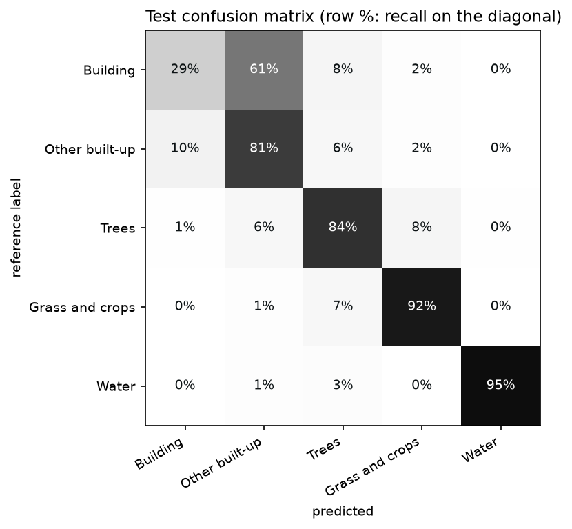

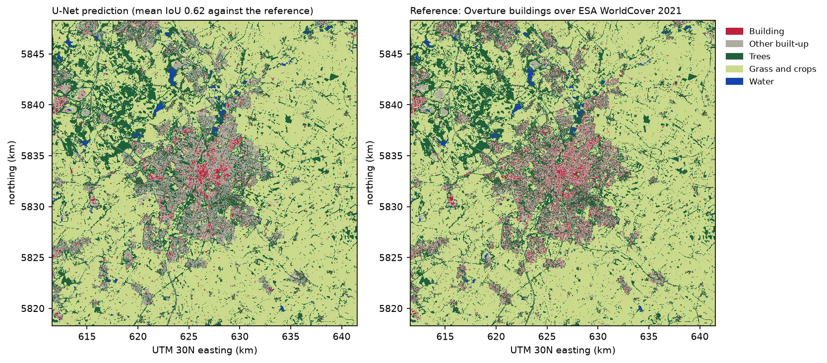
Almost all the building errors stay inside the built-up area: 61% of building pixels are predicted as other built-up, and 10.5% of other built-up pixels are predicted as buildings. The model knows where the town is, but it cannot reliably separate roofs from the roads, yards and gardens between them. Three things limit it, and none of them is solved by a bigger network:

1. Resolution. Sentinel-2’s 10 m pixel is about the size of a semi-detached house. A terraced street is a one-pixel stripe of roof beside a one-pixel stripe of road, and the bands at 20 m (red edge, SWIR) are even coarser.
2. Label noise at 10 m. In the test chips, only 88.8% of pixels have the same label as the pixel to their right. Much of that is real edges, but it also shows how much the labels depend on exactly where footprints fall within each pixel and on the 50% coverage threshold from part 1.
3. Mismatched dates. The buildings come from 2026 and the imagery from 2021, so new estates are labelled but not visible. WorldCover’s own errors, such as hedgerows as trees or fields as grassland, are also learned as if they were true.

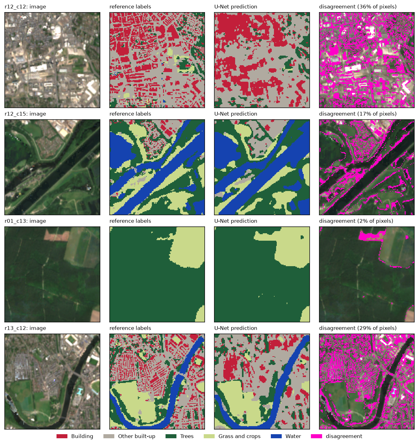
The predictions also show something the scores hide: the model’s buildings are smooth blobs over dense commercial areas, not individual roofs. For individual buildings, you need imagery at 1 m or finer. See Segment Anything on aerial imagery or building footprints from LiDAR.

Step 7: save the model for part 3

The checkpoint holds the weights and everything needed to use them: the architecture, the class names and colours, the band order, where the blank B10 goes and the scaling. Part 3 reads all of this from the file, so the two scripts cannot drift apart.

torch.save({"state_dict": model.state_dict(), "arch": "Unet", "encoder": "resnet18", "in_channels": 13,
            "classes": CLASSES, "colours": COLOURS, "bands": BANDS, "b10_zero_index": 10, "scale": 10000,
            "chip": int(X.shape[-1]), "test_scores": res.to_dict()}, ckpt)

saved unet_resnet18_s2_nottingham.pt (58 MB)

Limitations

• One city and one summer. The model has seen 416 chips of Nottingham in 2021. Expect it to be weaker in other landscapes, such as uplands or the coast, and in other seasons. Part 3 measures the drop in a new city.
• The labels are maps, not ground truth. The scores measure agreement with WorldCover and Overture, including their errors and their 2021 to 2026 date mismatch. A hand-labelled test set would give a truer accuracy.
• Buildings at 10 m. A building IoU of 0.21 is not useful for mapping individual buildings. Treat this model as a land cover mapper with a “dense roofs” class.
• Single runs. Each configuration was trained once, with one seed. Differences of 0.01 in mean IoU, such as pretrained against scratch, are within the variation you would see between seeds.
• CPU-sized choices. Small chips, 30 epochs and a ResNet-18 keep training to minutes. With a GPU, try 256-pixel chips, a ResNet-50 encoder with TorchGeo’s Sentinel-2 weights, and more epochs.

Frequently asked questions

Can I train a U-Net on satellite imagery without a GPU?

Yes, if you keep it small. Our U-Net with a ResNet-18 encoder took 4.8 minutes for 30 epochs over 416 chips of 128 × 128 pixels on 8 CPU threads, including a validation pass after every epoch. Training time grows with chip area, encoder size and epochs, so 256-pixel chips with a ResNet-50 would be roughly ten times slower. That is still feasible overnight on a CPU.

What is TorchGeo, and do I need it to train a U-Net?

TorchGeo is a PyTorch library for geospatial data. It adds datasets that read GeoTIFFs by location, spatial samplers, benchmark datasets and, most usefully here, encoders pretrained on Sentinel-1, Sentinel-2, Landsat and aerial imagery. You can train a U-Net without it, but its Sentinel-2 weights are the easiest way to start from an encoder that has seen multispectral satellite data rather than photographs.

Should I use ImageNet weights for Sentinel-2?

ImageNet weights expect three RGB bands with photograph statistics, so you either drop most of Sentinel-2’s bands or adapt the first layer. Weights pretrained on Sentinel-2 itself, such as TorchGeo’s SSL4EO-S12 weights, accept all 13 bands directly. In our run they trained more smoothly than random weights, but gave only a small final gain.

What is a good IoU for satellite image segmentation?

It depends on the class and resolution. For broad land cover at 10 m, IoUs of 0.7 to 0.9 for water, woodland and farmland are typical, and our model scored 0.71 to 0.88. Small objects at the limit of the resolution, such as houses in Sentinel-2, often stay below 0.3. Always compare against a simple baseline and report per-class scores on a spatially separate test set, not just overall accuracy.

Why use cross-entropy plus Dice loss?

Cross-entropy trains each pixel independently and, with class weights, copes reasonably well with imbalance. Dice loss measures the overlap for each class as a whole, so a rare class such as water counts as much as a common one. The combination is a robust default for multi-class segmentation of imbalanced land cover.

How do I run the trained model on a whole satellite image?

Split the image into overlapping windows, predict each window and blend the overlaps so the tile edges do not show. Part 3 does this over a 30 km Sentinel-2 composite of Leicester. It writes the result as a Cloud Optimised GeoTIFF and vectorises it to a GeoPackage.

Next steps

• Run the model over a new city with sliding-window inference in Part 3: deep learning inference on large rasters.
• Rebuild or extend the dataset, for example with another city or season, in Part 1: training data from Sentinel-2.
• Compare with a random forest on the same kind of labels in Land cover classification with a Sentinel-2 random forest.
• For individual buildings, use higher-resolution data: Segment Anything on aerial imagery or building footprints from LiDAR.

Data and licences

• Sentinel-2 L2A: Copernicus Sentinel data 2021, processed by ESA, accessed from the Microsoft Planetary Computer. Free and open under the Copernicus data licence.
• ESA WorldCover 2021 (v200): © ESA WorldCover project 2021, contains modified Copernicus Sentinel data (2021) processed by the ESA WorldCover consortium. CC BY 4.0.
• Building footprints: Overture Maps Foundation, release 2026-09-23.1, under the ODbL. Contains data © OpenStreetMap contributors and Microsoft ML Buildings.
• Pretrained weights: TorchGeo ResNet18_Weights.SENTINEL2_ALL_MOCO, from Wang, Y. et al. (2023), SSL4EO-S12: A large-scale multimodal, multitemporal dataset for self-supervised learning in Earth observation, IEEE Geoscience and Remote Sensing Magazine. Released under CC BY 4.0. TorchGeo is MIT-licensed; segmentation_models_pytorch is MIT-licensed.
• Code: train_unet.py, tested with Python 3.12.0, PyTorch 2.14.1 (CPU), segmentation-models-pytorch 0.5.0, TorchGeo 0.10.1, timm 1.0.30 and rasterio 1.5.2.