Object-based image analysis in Python: OBIA habitat classification with Sentinel-2
Segment 2023 Sentinel-2 seasonal composites of the Peak District into image objects with scikit-image SLIC and Felzenszwalb, tune the segment size against Living England boundaries, compute per-object statistics, shape and GLCM texture with NumPy, classify the objects with LightGBM and compare OBIA with a pixel-based classifier on accuracy, salt-and-pepper noise and patch counts. Then export the habitat objects as GeoPackage polygons.
- Level
- Advanced
- Tested with
- Python 3.12
- Source code
- Download scripts
Key takeaways
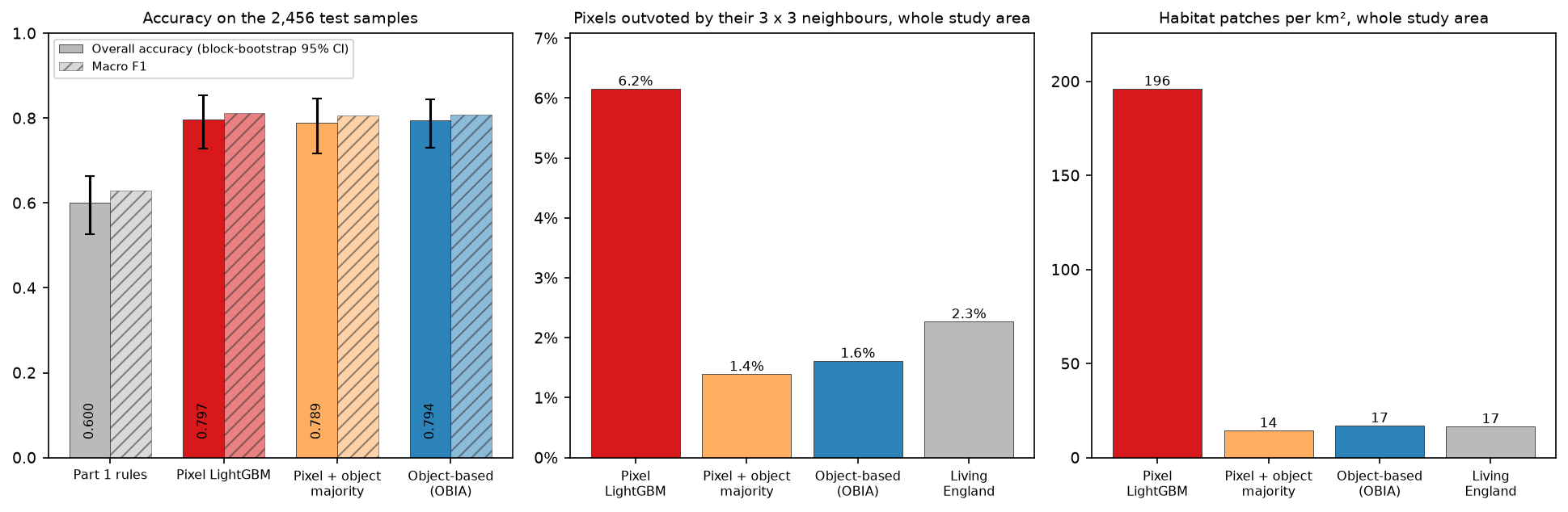
- Felzenszwalb segments of about 0.6 ha, chosen by blocked cross-validation, classified with LightGBM give 79.4% overall accuracy on the shared test blocks (95% CI 72.9% to 84.5%) and macro F1 0.81, against 60.0% for Part 1's rules.
- A pixel-based LightGBM on the same 52 seasonal features scores the same (79.7%). OBIA does not buy accuracy here; it buys clean maps.
- The pixel map has 196 habitat patches per km² and 6.2% of pixels outvoted by their 3 × 3 neighbours. The object map has 17 per km² and 1.6%, close to Living England's 17 and 2.3%.
- Smaller objects scored best. Mean object values and within-object percentiles do the work; shape adds little and GLCM texture adds nothing at 10 m.
- Classifying pixels and then taking a majority vote in each object is a cheap alternative with very similar results.
Before you start
- Part 1 of this series, Habitat mapping with Sentinel-2 in Python, for the study area, labels, spatial split and seasonal composites (you do not need to run its code)
- Python with NumPy and pandas; some familiarity with a tree-based classifier such as random forest or LightGBM
- Python 3.12 with scikit-image, LightGBM, rasterio, geopandas and the series' shared module (see requirements.txt); about 8 GB of RAM, no GPU
Short answer: to do object-based image analysis (OBIA) in Python, segment a multi-band image into objects with scikit-image (slic or felzenszwalb). Then aggregate each pixel layer per object with np.bincount on the segment labels to get means, spreads, percentiles, shape and texture. Train a classifier such as LightGBM on the objects that contain training samples, predict every object, and paint the class back onto the pixels or polygonise the objects to a GeoPackage. Choose the segment size by cross-validation, not by eye. In the Dark Peak, OBIA on Sentinel-2 matches a pixel-based classifier’s accuracy (79.4% against 79.7%) and cuts the number of habitat patches from 196 to 17 per km².
Pixel-based classifiers judge every 10 m pixel on its own. The result is a map that is right on average but speckled with isolated pixels of the wrong class: the salt-and-pepper effect. GIS users then struggle to turn it into the polygons that habitat surveys, Biodiversity Net Gain baselines and land management plans need. Object-based image analysis groups similar neighbouring pixels into objects first and classifies the objects. Each object gets one label and can use statistics that a single pixel does not have: its spread of values, its size and shape, and its texture.
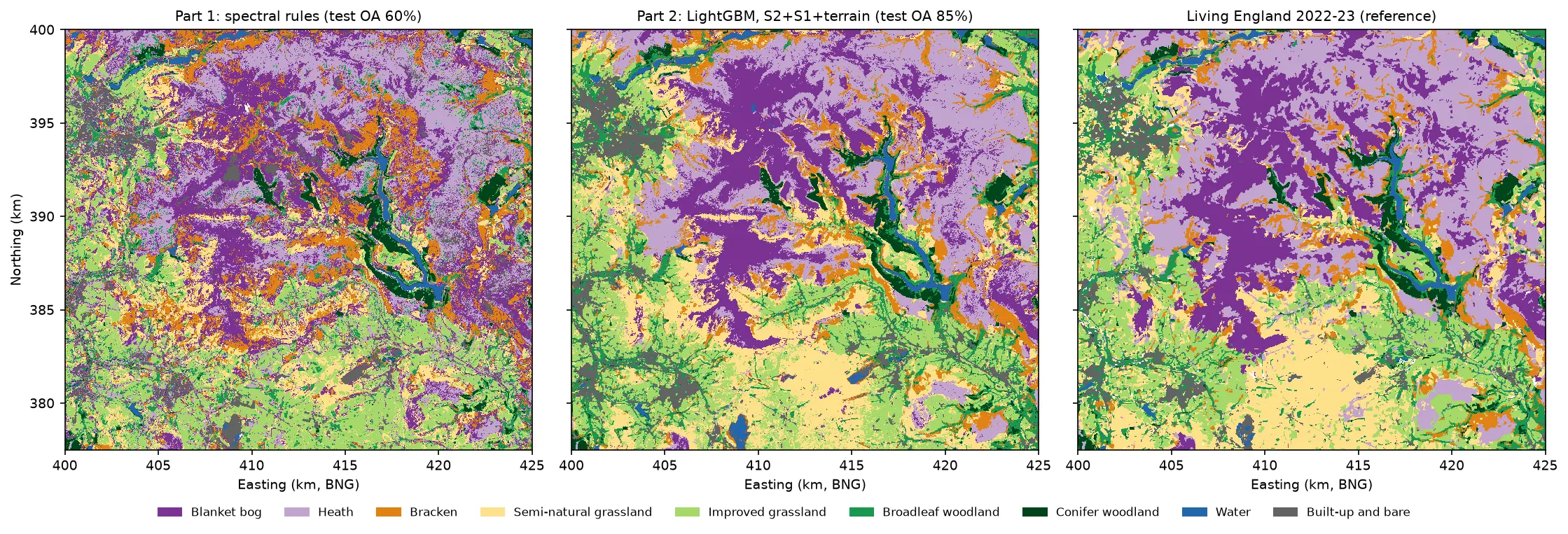
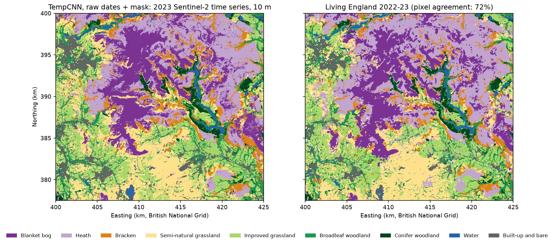
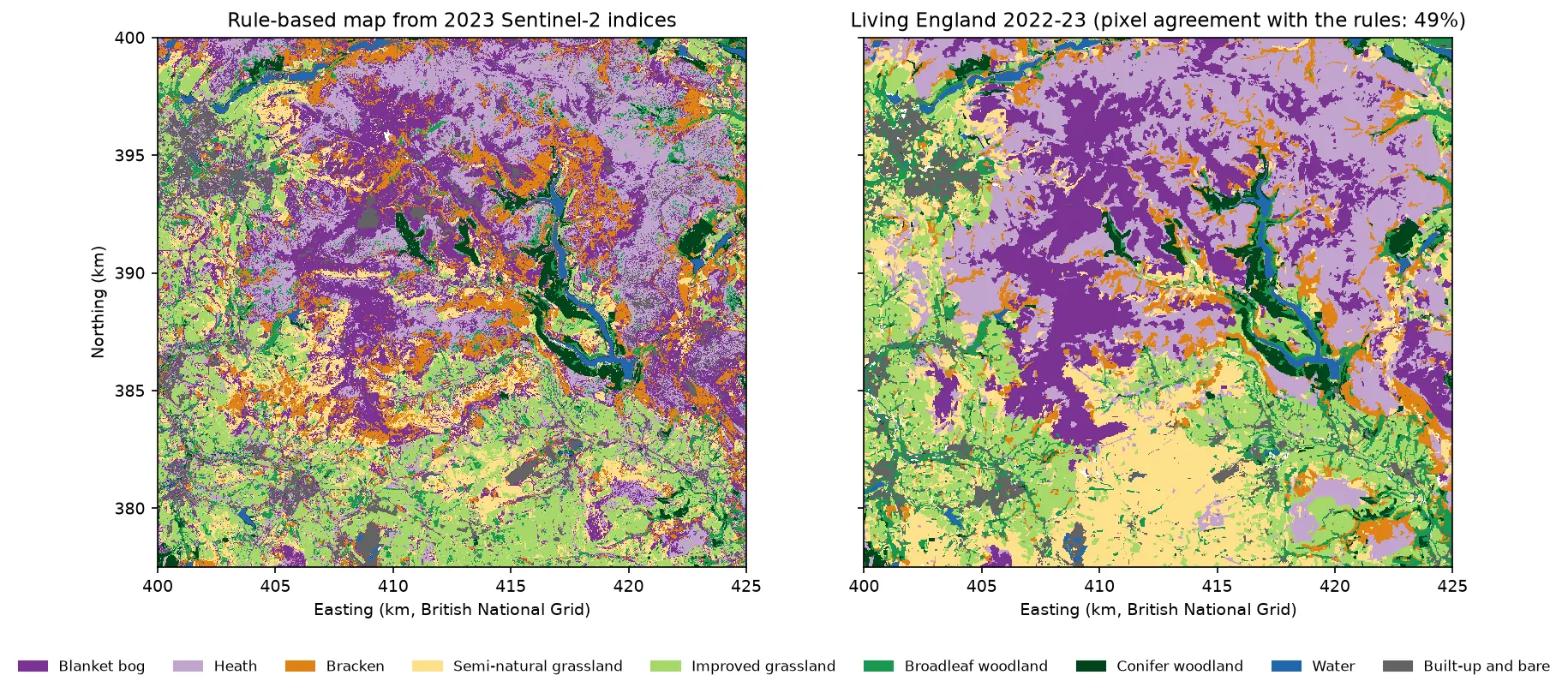
This is part 3 of the five-part series AI habitat classification with Python. Every part maps the same nine habitats in the Dark Peak of the Peak District, with labels from Natural England’s Living England map and the same spatial train/test split, so the accuracies compare directly. Part 1 built the study area, labels, split and seasonal composites, and set a baseline of 60.0% overall accuracy with spectral index rules. Part 2 trains LightGBM on pixel features from Sentinel-2 and Sentinel-1. This part does not depend on Part 2: it trains its own pixel-based LightGBM on the same seasonal Sentinel-2 features as a fair comparison for the objects.
You will learn how to:
- segment a Sentinel-2 composite into objects with SLIC and Felzenszwalb in scikit-image;
- tune the segment size with boundary recall, achievable accuracy and blocked cross-validation;
- compute object features (statistics, percentiles, shape and GLCM texture) for 90,000 objects with NumPy;
- classify objects with LightGBM and evaluate them on the same test pixels as a pixel-based map;
- measure salt-and-pepper noise with a 3 × 3 majority test and patch counts;
- export habitat polygons to a GeoPackage for QGIS or ArcGIS.
All outputs below come from obia_habitat.py and the series’ shared module and sample design (habitat_common.py, prepare_data.py and the sample CSVs). They were run on 21 October 2026 with Python 3.12, scikit-image 0.26.0, LightGBM 4.7.0, NumPy 2.5.4, rasterio 1.5.2 and geopandas 1.2.0, on a 32-thread desktop with no GPU. The full script took 9.5 minutes, most of it spent trying twelve segmentations.
Setting up: the shared data in one command
You do not need to run Part 1. Create the series environment from this tutorial’s requirements.txt (the shared pins plus scikit-image and LightGBM), then build the labels and the seasonal composites with the series’ shared script:
python -m venv .venv-habitat.venv-habitat\Scripts\activate # source .venv-habitat/bin/activate on Linux or macOSpip install -r tutorial-code/object-based-image-analysis-python/requirements.txtpython tutorial-code/ai-habitat-classification-common/prepare_data.py --compositespython tutorial-code/object-based-image-analysis-python/obia_habitat.pyprepare_data.py --composites downloads the Living England polygons, rasterises them to the 10 m grid on the British National Grid and builds cloud-masked median composites of Sentinel-2 for winter, spring, summer and autumn 2023 from the Microsoft Planetary Computer. It also builds Sentinel-1 composites, which this part does not use. The 9,000 sample pixels (1,000 per class) and the 90 blocks of 2.5 km, 27 of which are held out for testing, are committed to the repository.
The script loads them through the shared module and stacks 52 pixel features: the ten 10 m and 20 m bands plus NDVI, NDMI and NDWI for each season.
import habitat_common as hc                      # the series' shared module
labels = hc.label_raster()                       # Living England 2022-23 on the 10 m grid (0 = unlabelled)samples = hc.load_samples()train_s, test_s = samples[samples.split == "train"], samples[samples.split == "test"]S = hc.s2_seasonal_composites()                  # {"winter", "spring", "summer", "autumn"} -> Datasetrr, cc = np.indices((ROWS, COLS))BLK = (rr // 250) * 10 + cc // 250               # 2.5 km block of every pixel (same ids as hc.block_id)
FEAT = {}for s, ds in S.items(): b = {k: ds[k].values.astype("float32") for k in hc.S2_BANDS} FEAT.update({f"{k}_{s}": b[k] for k in hc.S2_BANDS}) FEAT[f"ndvi_{s}"] = nd(b["B08"], b["B04"]) FEAT[f"ndmi_{s}"] = nd(b["B08"], b["B11"]) FEAT[f"ndwi_{s}"] = nd(b["B03"], b["B08"])FNAMES = list(FEAT)F = np.stack([FEAT[k] for k in FNAMES]) # (52, rows, cols)6,544 training and 2,456 test samples; grid 2500 x 2250 pixels at 10 m52 pixel feature layers (1.17 GB in memory)Step 1: segment the image into objects
Segmentation needs a few layers that show the boundaries we care about, scaled to a common range. We use six: spring and summer NDVI (vegetation and its seasonal change, which separates bracken), spring NDMI (moisture, which separates moorland from grassland), and summer near-infrared, shortwave infrared and red. Each is stretched between its 2nd and 98th percentiles to 0–1.
scikit-image offers two fast segmentations that work well on multi-band rasters:
- SLIC (simple linear iterative clustering) runs k-means in a space of band values plus position. It gives compact superpixels of roughly equal size. You set the number of segments, so we convert a target mean size in hectares into
n_segments.compactnesstrades spectral fit against regular shape; with 0–1 scaled bands, 0.1 lets objects follow field edges. - Felzenszwalb grows a minimum spanning tree over a pixel graph and merges regions whose internal difference is small compared with the difference between them.
scalecontrols how readily regions merge, so larger values make larger objects, and objects vary in size: big where the land is uniform, small where it is varied.
from skimage.segmentation import felzenszwalb, slic
def cut_by_blocks(seg):    """Split any object that crosses a 2.5 km block edge, so no object is shared by training and test blocks."""    key = seg.astype(np.int64) * 100 + BLK    u, inv = np.unique(key.ravel(), return_inverse=True)    return inv.reshape(seg.shape).astype(np.int32), len(u)

def segment(method, param):    if method == "slic":                         # param = target mean object size in hectares        seg = slic(IMG, n_segments=int(ROWS * COLS / (param / PX_HA)), compactness=0.1, channel_axis=-1,                   convert2lab=False, start_label=0)    else:                                        # param = Felzenszwalb scale (larger = bigger objects)        seg = felzenszwalb(IMG, scale=param, sigma=0.5, min_size=20, channel_axis=-1)    return cut_by_blocks(seg)
cut_by_blocks matters for honest evaluation. Without it, one object could straddle a training block and a test block, and the test pixels in it would share their features with training samples. Cutting objects at block edges keeps the split as clean as in Part 1, at the cost of some straight object edges along the 2.5 km grid. Use convert2lab=False because the image is not RGB, and channel_axis=-1 to treat the six layers as one multi-channel image.
Each segmentation of the full 25 × 22.5 km area (5.6 million pixels) takes about 5 seconds with SLIC and 10–13 seconds with Felzenszwalb.
Step 2: tune the segment size against Living England
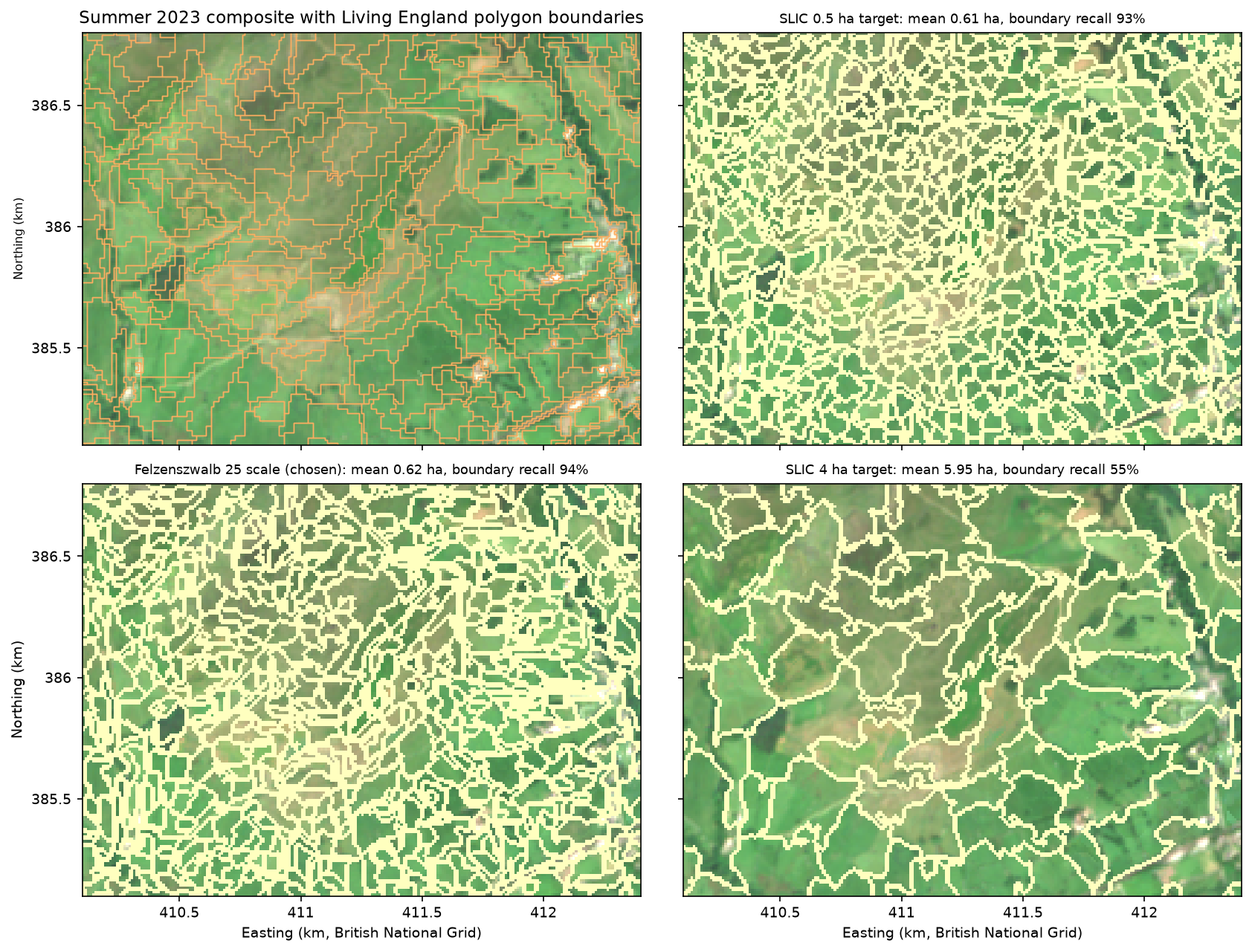
Segment size is the main OBIA decision. Objects that are too large merge different habitats, and no classifier can split them again. Objects that are too small bring back the noise that OBIA is meant to remove and have unreliable statistics. We scored twelve candidates, six sizes for each method, in three ways, using only the training blocks:
- Boundary recall: the share of Living England class boundary pixels with an object edge within 10 m (one pixel). This is a standard under-segmentation check: low recall means objects cross real boundaries.
- Achievable segmentation accuracy (ASA): the agreement with Living England if every object took its majority Living England class. It is the ceiling that the segmentation puts on any classifier.
- Blocked 5-fold cross-validation (CV) of the full object classifier (Step 4), scored on the training samples. This is what we choose by, because it is what we care about.
LE_EDGE = edges(labels) & train_px & ~near_block_edge   # Living England class boundaries (both sides, 1 px)
def segmentation_quality(seg, n): """Boundary recall (LE boundaries within 10 m of an object edge) and achievable segmentation accuracy (ASA).""" recall = (LE_EDGE & ndimage.binary_dilation(edges(seg), np.ones((3, 3), bool))).sum() / LE_EDGE.sum() cm = np.bincount(seg[train_px].astype(np.int64) * 10 + labels[train_px], minlength=n * 10).reshape(n, 10) asa = cm.max(1).sum() / cm.sum() # best wall-to-wall agreement if every object took its majority class return recall, asaslic 0.25 192,643 objects, mean 0.29 ha boundary recall 0.983 ASA 0.910 blocked CV OA 0.834 +/- 0.017 (6 s)slic 0.5 91,765 objects, mean 0.61 ha boundary recall 0.927 ASA 0.881 blocked CV OA 0.830 +/- 0.016 (5 s)slic 1 41,911 objects, mean 1.34 ha boundary recall 0.821 ASA 0.842 blocked CV OA 0.811 +/- 0.021 (6 s)slic 2 20,521 objects, mean 2.74 ha boundary recall 0.696 ASA 0.798 blocked CV OA 0.791 +/- 0.013 (5 s)slic 4 9,456 objects, mean 5.95 ha boundary recall 0.550 ASA 0.747 blocked CV OA 0.766 +/- 0.016 (5 s)slic 8 4,556 objects, mean 12.35 ha boundary recall 0.420 ASA 0.695 blocked CV OA 0.695 +/- 0.032 (5 s)felzenszwalb 10 80,564 objects, mean 0.70 ha boundary recall 0.926 ASA 0.883 blocked CV OA 0.839 +/- 0.016 (10 s)felzenszwalb 25 90,267 objects, mean 0.62 ha boundary recall 0.943 ASA 0.888 blocked CV OA 0.842 +/- 0.013 (11 s)felzenszwalb 50 78,284 objects, mean 0.72 ha boundary recall 0.936 ASA 0.880 blocked CV OA 0.834 +/- 0.021 (13 s)felzenszwalb 100 50,985 objects, mean 1.10 ha boundary recall 0.878 ASA 0.846 blocked CV OA 0.828 +/- 0.020 (11 s)felzenszwalb 200 28,017 objects, mean 2.01 ha boundary recall 0.782 ASA 0.793 blocked CV OA 0.805 +/- 0.023 (10 s)felzenszwalb 400 14,780 objects, mean 3.81 ha boundary recall 0.652 ASA 0.716 blocked CV OA 0.731 +/- 0.029 (12 s)chosen by blocked CV: felzenszwalb 25 (90,267 objects, mean 0.62 ha)object size: median 0.50 ha, 5th-95th percentile 0.16-1.48 ha; 151 features per object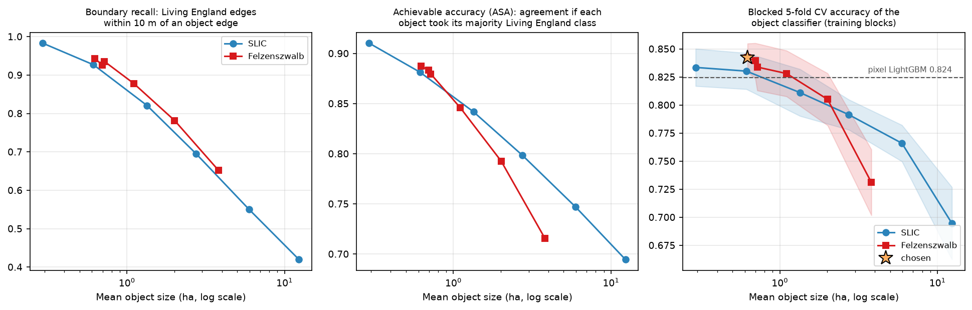
Three things stand out:
- Small objects win. Every measure falls as objects grow. Cross-validated accuracy is flat between 0.3 and 1 ha and drops quickly beyond 2 ha: 8 ha SLIC objects lose 15 points. Upland habitats form a fine mosaic (bracken on a slope, a strip of woodland along a clough), and Sentinel-2’s 10 m pixels are already coarse for it.
- Felzenszwalb beats SLIC at the same mean size, with higher boundary recall and CV accuracy, because its objects can be large on uniform moorland and small in the fields. The differences between the best few candidates (0.834 to 0.842) are well within one standard deviation across folds, so any of them would do.
- Felzenszwalb’s
scaleis not a size dial at small values. Withmin_size=20, scale 10 gives fewer objects than scale 25, because many tiny regions are merged into neighbours at the end. Check the object count, not just the parameter.
Step 3: object features with NumPy label aggregation
With a label image seg (one integer per object), per-object statistics are just grouped sums. np.bincount(seg.ravel(), weights=values) adds up a layer’s values for every object in one pass, which is far faster than looping over objects. It is the same idea as zonal statistics in Python, with the segments as zones. For polygons from a file, exactextract or rasterstats would do the job, but here the zones are already a raster on the same grid.
For each object we compute:
- mean and standard deviation of all 52 layers (sums and sums of squares per object, ignoring cloud gaps);
- the 10th, 50th and 90th percentiles of 11 key layers: NDVI and NDMI in every season, summer near-infrared and shortwave infrared, and spring red. Sorting all pixels by object and then value with
np.lexsortgives each object’s sorted values as one contiguous run; - shape: area, perimeter, compactness (4πA/P², 1 for a circle) and elongation from second moments;
- GLCM texture inside each object, for summer near-infrared and spring NDVI.
def object_stats(seg, n): """Mean and standard deviation of every layer, and 10th/50th/90th percentiles of a subset, per object.""" flat = seg.ravel() cnt = np.bincount(flat, minlength=n) start = np.concatenate([[0], np.cumsum(cnt)[:-1]]) out = {} for i, name in enumerate(FNAMES): v = F[i].ravel() ok = ~np.isnan(v) nv = np.bincount(flat[ok], minlength=n) s1 = np.bincount(flat[ok], weights=v[ok], minlength=n) s2 = np.bincount(flat[ok], weights=v[ok].astype(float) ** 2, minlength=n) mean = s1 / nv out[f"{name}_mean"] = mean out[f"{name}_std"] = np.sqrt(np.maximum(s2 / nv - mean ** 2, 0)) if name in PCTL_LAYERS: sv = v[np.lexsort((v, flat))] # sorted by object, then value (NaN last within each object) for q in (10, 50, 90): k = start + np.floor(q / 100 * np.maximum(nv - 1, 0)).astype(int) out[f"{name}_p{q}"] = np.where(nv > 0, sv[np.minimum(k, flat.size - 1)], np.nan) return outTexture uses the grey-level co-occurrence matrix (GLCM), which counts how often each pair of grey levels occurs in neighbouring pixels. skimage.feature.graycomatrix computes one GLCM per image, which would mean 90,000 calls. Instead we quantise the layer to 16 levels and count (object, level, neighbour level) triples for all objects with a single bincount, using only pixel pairs where both pixels are in the same object:
def object_glcm(seg, n, name, levels=16): a = F[FNAMES.index(name)] edges = np.nanpercentile(a, np.linspace(0, 100, levels + 1)[1:-1]) q = np.digitize(a, edges).astype(np.int64) q[np.isnan(a)] = -1 counts = np.zeros(n * levels * levels, np.int64) for (sa, sb), (qa, qb) in (((seg[:, :-1], seg[:, 1:]), (q[:, :-1], q[:, 1:])), # horizontal pairs ((seg[:-1, :], seg[1:, :]), (q[:-1, :], q[1:, :]))): # vertical pairs same = (sa == sb) & (qa >= 0) & (qb >= 0) counts += np.bincount((sa[same].astype(np.int64) * levels + qa[same]) * levels + qb[same], minlength=n * levels * levels) P = counts.reshape(n, levels, levels).astype(float) P = P + P.transpose(0, 2, 1) # symmetric GLCM P = P / P.sum((1, 2), keepdims=True) # (the script guards empty objects) i, j = np.meshgrid(np.arange(levels), np.arange(levels), indexing="ij") contrast = (P * (i - j) ** 2).sum((1, 2)) homogeneity = (P / (1 + (i - j) ** 2)).sum((1, 2)) ... # entropy, angular second moment and correlation likewiseThat gives 151 features for each of the 90,267 objects. Which ones matter? We added the families one at a time and reran the blocked CV:
Spectral mean only 52 features CV OA 0.825 +/- 0.018+ spread and percentiles 137 features CV OA 0.839 +/- 0.014+ shape 141 features CV OA 0.842 +/- 0.011+ texture (all features) 151 features CV OA 0.842 +/- 0.013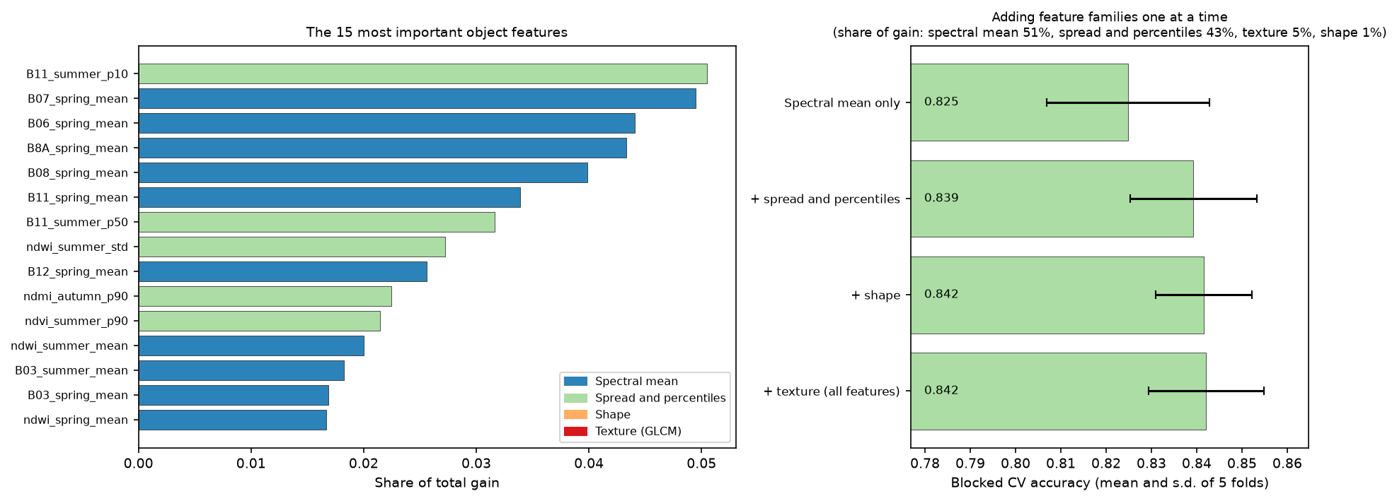
The within-object distribution adds 1.4 points: the 10th percentile of summer shortwave infrared is the single most important feature, and percentiles are robust to the mixed pixels at object edges. Shape adds 0.3 points, within the fold-to-fold noise. Texture adds nothing. At 10 m a typical 0.5 ha object has only 50 pixels, too few for a stable texture estimate, and the textures that separate habitats (heather burning patterns, tussocks, tree crowns) are finer than a pixel. GLCM texture earns its keep on aerial imagery, not on Sentinel-2.
Step 4: classify the objects
The training data are the objects that contain training samples. Each takes the majority class of its samples. The classifier is LightGBM with modest, fixed settings; a random forest gives similar results.
PARAMS = dict(n_estimators=300, learning_rate=0.05, num_leaves=15, min_child_samples=10, subsample=0.8,              subsample_freq=1, colsample_bytree=0.5, reg_lambda=1.0, random_state=hc.SEED, verbose=-1)
def training_objects(seg, smp):    """One row per object that contains training samples: its majority sample class and its block fold."""    df = pd.DataFrame({"obj": seg[smp.row, smp.col], "cls": smp.class_id.to_numpy(), "fold": smp.fold.to_numpy()})    return df.groupby("obj").agg(cls=("cls", lambda s: s.mode().iloc[0]), fold=("fold", "first"), n=("cls", "size"))
g = training_objects(seg, train_s)obj_model = lgb.LGBMClassifier(**PARAMS).fit(OF.loc[g.index], g.cls)proba = obj_model.predict_proba(OF) # every object in the study areaobj_class = obj_model.classes_[proba.argmax(1)].astype("uint8")obj_conf = proba.max(1)obia_map = obj_class[seg] # paint each object's class onto its pixels6,544 training samples fall in 5,260 objects (887 objects hold more than one sample)trained on 5,260 objects and classified 90,267 objects in 3.0 sTwo details matter. First, samples that share an object are not independent: 887 objects hold two or more samples, so the effective training set is 5,260 objects, not 6,544 pixels. Second, obj_class[seg] uses the object IDs as an index array, which turns 90,267 object predictions into a 5.6 million pixel map in one step.
Step 5: a pixel-based comparison on the same features
To see what OBIA changes, we need a pixel-based map made the same way. We train the same LightGBM on the 52 pixel values at the 6,544 training samples and predict every pixel. We also try a common shortcut: classify pixels, then give every object the majority vote of its pixels.
Xp = hc.sample_values(F, train_s)                         # (6,544, 52) pixel featurespix_model = lgb.LGBMClassifier(**PARAMS).fit(Xp, train_s.class_id)pix_map = np.zeros((ROWS, COLS), "uint8")for r0 in range(0, ROWS, 250):                            # predict in strips to limit memory    chunk = F[:, r0:r0 + 250].reshape(len(FNAMES), -1).T    pix_map[r0:r0 + 250] = pix_model.predict(chunk).reshape(-1, COLS)
votes = np.bincount(seg.ravel().astype(np.int64) * 10 + pix_map.ravel(), minlength=n_obj * 10).reshape(n_obj, 10)vote_map = votes[:, 1:].argmax(1).astype("uint8")[seg] + 1trained on 6,544 pixels and classified 5,625,000 pixels in 60.2 spixel blocked CV OA 0.824 +/- 0.020 (objects: 0.842 +/- 0.013)Note the cost: predicting 5.6 million pixels takes a minute, against 3 seconds for 90,000 objects.
Step 6: accuracy on the shared test pixels
The series compares methods on the same 2,456 test pixels in 27 held-out blocks. For OBIA, each test pixel takes the class of the object it falls in, which is simply the map value at its location. That puts pixel and object maps on exactly the same footing.
def evaluate(pred_map, name): """Accuracy at the shared test samples: each test pixel takes the class of the map at its location.""" yt = test_s.class_key.to_numpy() yp = np.array([ID_KEY.get(v, "none") for v in pred_map[test_s.row, test_s.col]]) cm = confusion(yt, yp) res = summarise(cm) # OA, kappa, per-class PA, UA and F1 res["ci"] = block_bootstrap(yt == yp, test_s.block_id.to_numpy()) ...Pixel LightGBM OA 0.797 (95% CI 0.728-0.853) macro F1 0.812 kappa 0.769 wall-to-wall (test blocks) 0.635Pixel LightGBM + object majority OA 0.789 (95% CI 0.716-0.847) macro F1 0.806 kappa 0.761 wall-to-wall (test blocks) 0.643Object-based LightGBM (OBIA) OA 0.794 (95% CI 0.729-0.845) macro F1 0.808 kappa 0.766 wall-to-wall (test blocks) 0.642Part 1 baseline (spectral rules) OA 0.600 (95% CI 0.527-0.664) macro F1 0.630 kappa 0.547 wall-to-wall (test blocks) 0.483All three machine learning maps are about 20 points better than Part 1’s rules, and they are indistinguishable from each other: the differences of 0.3 to 0.8 points are tiny next to the block-bootstrap intervals of about ±6 points. The objects had a 1.8 point lead in cross-validation, but it did not carry over to the test blocks. Wall-to-wall agreement with Living England across the test blocks, which counts every labelled pixel rather than the pure samples, is slightly higher for the object maps (64.2% against 63.5%).
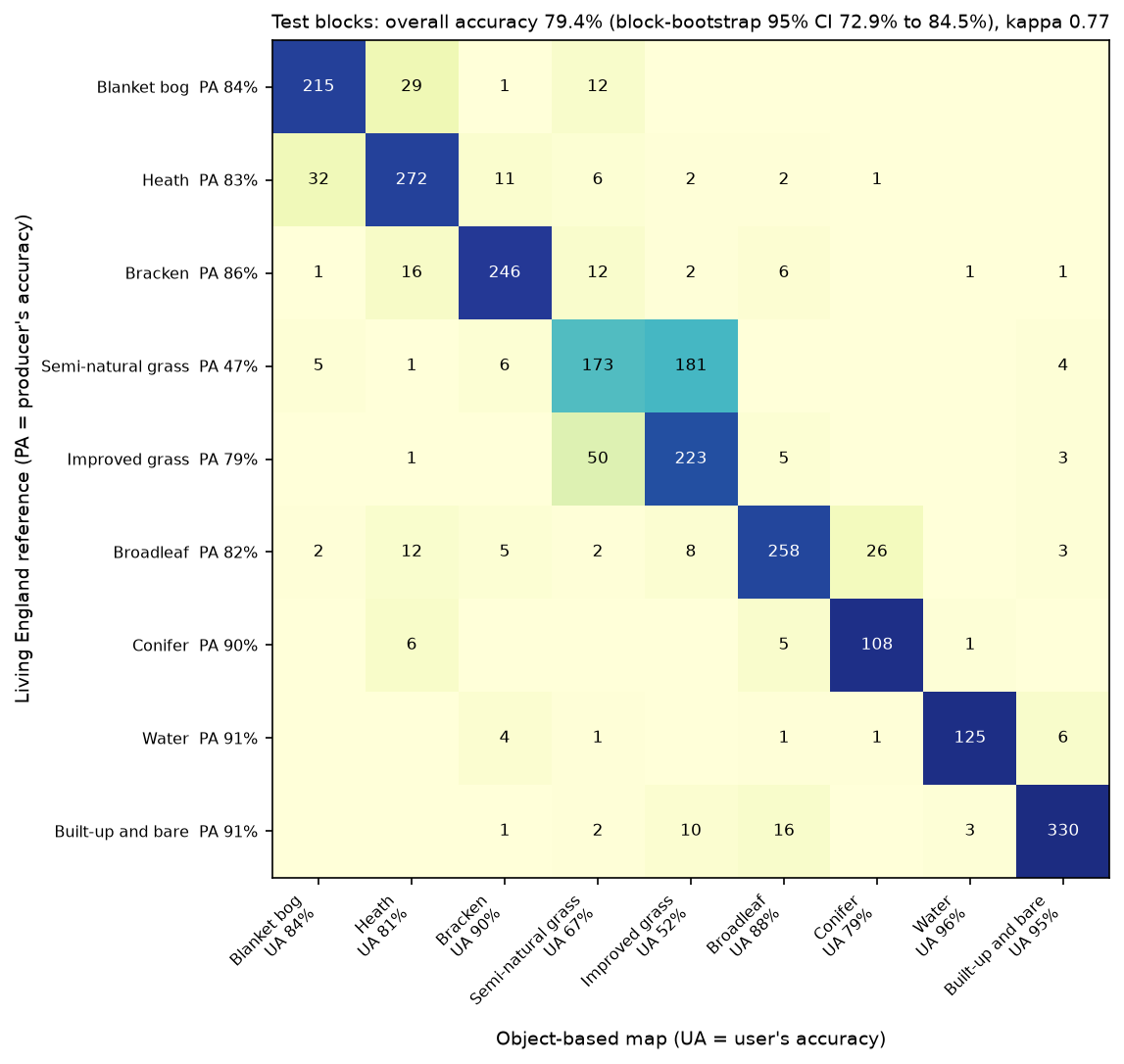
Per class, objects help where habitats form coherent patches and hurt where they form narrow strips:
| Class | Pixel F1 | OBIA F1 | Change |
|---|---|---|---|
| Blanket bog | 0.792 | 0.840 | +0.048 |
| Heath | 0.815 | 0.821 | +0.006 |
| Bracken | 0.853 | 0.880 | +0.027 |
| Semi-natural grassland | 0.548 | 0.551 | +0.003 |
| Improved grassland | 0.642 | 0.630 | −0.012 |
| Broadleaf woodland | 0.889 | 0.847 | −0.042 |
| Conifer woodland | 0.876 | 0.844 | −0.032 |
| Water | 0.951 | 0.933 | −0.018 |
| Built-up and bare | 0.941 | 0.931 | −0.010 |
Blanket bog and bracken gain most. Both are large, internally variable patches where averaging over an object removes noise and percentiles describe the mix of heather, cotton grass and bare peat. Broadleaf woodland and conifers lose most, because the woodland in the Dark Peak is mostly narrow strips along cloughs and reservoir shores, two or three pixels wide, which 0.5 ha objects merge with the fields beside them. That is the classic OBIA trade-off: the segment size suits the typical patch, not the narrowest one.
Semi-natural grassland is still the weak spot, as in Part 1. Unimproved and improved grassland are both green fields to Sentinel-2, and the difference (species richness and management history) is not something objects can see either.
Step 7: measuring the salt-and-pepper effect
Accuracy at sample points cannot see map noise, because the samples come from the middle of large, pure polygons. To measure it directly, we use two map-wide metrics:
- outvoted pixels: the share of pixels whose own class is not the most common class in their 3 × 3 neighbourhood. An isolated pixel is always outvoted; a pixel inside a patch never is;
- patches: the number of 8-connected regions of one class, per km². Every speck is a patch.
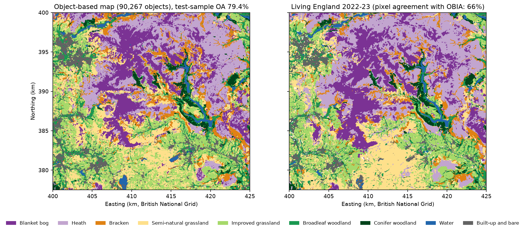
def noise(m): counts = np.stack([ndimage.uniform_filter((m == c).astype("float32"), 3, mode="nearest") for c in hc.CLASS_IDS]) own = np.take_along_axis(counts, (np.clip(m, 1, 9) - 1)[None].astype(np.int64), 0)[0] outvoted = (own < counts.max(0) - 1e-6) & (m > 0) patches = sum(ndimage.label(m == c, structure=np.ones((3, 3), bool))[1] for c in hc.CLASS_IDS) ... outvoted_3x3_% patches patches_per_km2 single_pixel_patches mean_patch_haLiving England (reference) 2.27 9300.0 16.59 6.0 6.03Pixel LightGBM 6.16 110332.0 196.15 45525.0 0.51Pixel + object majority 1.40 8097.0 14.39 65.0 6.95Object-based (OBIA) 1.62 9607.0 17.08 109.0 5.86The pixel map has 110,332 patches, of which 45,525 are single pixels, and 6.2% of its pixels are outvoted by their neighbours. The object map has 9,607 patches, a mean patch size of 5.9 ha and 1.6% outvoted pixels, almost exactly matching Living England, which is itself a segmentation-based product. The zoom shows what that means on the ground:
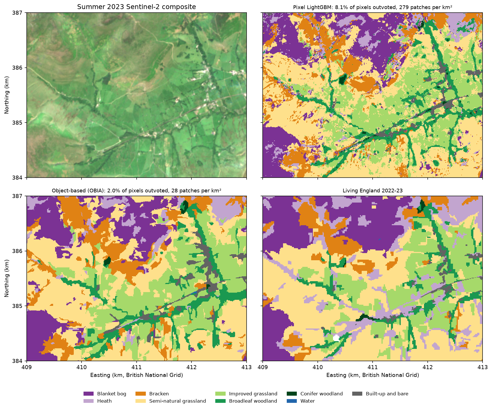
The pixel + object majority shortcut is just as clean, and its accuracy is within the noise of the full OBIA workflow. If you already have a pixel classifier, segmenting the image and taking a vote in each object is the cheapest way to get a clean map. Full OBIA is worth it when object statistics add information: here they helped bog and bracken, and they make classification 20 times faster because there are 60 times fewer things to predict.
Step 8: export habitat polygons to a GeoPackage
GIS users want polygons, not rasters. Because each object already has an ID, rasterio.features.shapes turns the segment raster into polygons, and we attach the class, the classifier’s confidence and a few object statistics. A second layer dissolves neighbouring objects of the same class into habitat patches.
from rasterio.features import shapesfrom shapely.geometry import shape as as_shape
geoms, ids = zip(*((as_shape(gm), int(v)) for gm, v in shapes(seg, transform=hc.transform())))gdf = gpd.GeoDataFrame({"object_id": np.array(ids, "int32")}, geometry=list(geoms), crs=hc.CRS)gdf = gdf.dissolve("object_id", as_index=False)  # an object cut by a block edge can have two partsids = gdf.object_id.to_numpy()gdf["class_id"] = obj_class[ids]gdf["habitat"] = [NAMES[ID_KEY[v]] for v in gdf.class_id]gdf["confidence"] = obj_conf[ids].round(3)gdf["area_ha"] = OF.area_ha.to_numpy()[ids].round(2)gdf.to_file("output/habitat_obia_2023.gpkg", layer="habitat_objects", driver="GPKG")
geoms, vals = zip(*((as_shape(gm), int(v)) for gm, v in shapes(obia_map, mask=obia_map > 0, transform=hc.transform())))patches = gpd.GeoDataFrame({"class_id": np.array(vals, "uint8")}, geometry=list(geoms), crs=hc.CRS)patches.to_file("output/habitat_obia_2023.gpkg", layer="habitat_patches", driver="GPKG")90,267 object polygons and 20,186 dissolved habitat patches written to habitat_obia_2023.gpkg (87 MB) in 10 s object_id class_id class_key habitat confidence area_ha ndvi_summer_mean block_split 0 2 heath Heath 0.975 0.29 0.640 test 1 2 heath Heath 0.998 0.95 0.694 test 2 2 heath Heath 0.942 0.48 0.693 testOpen the GeoPackage in QGIS, style habitat by category and filter confidence < 0.6 to find the objects worth checking in the field. The polygon edges follow the 10 m pixel grid; if you need smoother lines for display, simplify them with gdf.simplify(5), but keep the originals for area statistics. The block_split column flags objects in the test blocks, so you can summarise accuracy or area by split.
The series so far
| Measure (test blocks, n = 2,456) | Part 1: spectral rules | Part 3: pixel LightGBM | Part 3: OBIA |
|---|---|---|---|
| Overall accuracy (95% CI) | 0.600 (0.527 to 0.664) | 0.797 (0.728 to 0.853) | 0.794 (0.729 to 0.845) |
| Macro F1 | 0.630 | 0.812 | 0.808 |
| Cohen’s kappa | 0.547 | 0.769 | 0.766 |
| Blocked 5-fold CV on training blocks | 0.684 ± 0.030 | 0.824 ± 0.020 | 0.842 ± 0.013 |
| Wall-to-wall agreement, test blocks | 0.483 | 0.635 | 0.642 |
| Patches per km² (Living England: 16.6) | not measured | 196 | 17 |
| Hardest class (F1) | Semi-natural grassland 0.33 | Semi-natural grassland 0.55 | Semi-natural grassland 0.55 |
The pixel LightGBM here uses Sentinel-2 seasonal features only. Part 2 adds Sentinel-1 radar and terrain and studies its features in depth; Part 4 and Part 5 try a temporal neural network and foundation-model embeddings on the same split. The five-method comparison in Part 5 puts all the results side by side.
Limitations
- The labels are a model. Living England is a classification with its own errors, so these numbers measure agreement with it, not with field survey. It is also object-based itself, which may flatter object maps in the wall-to-wall and patch-count comparisons.
- Balanced, pure samples. Test pixels come from the middle of reliable polygons, where objects are easy. Mixed pixels at boundaries, where OBIA and pixel methods differ most, are under-represented, so sample accuracy says little about edges. Use area-weighted accuracy (Part 5) for a map product.
- Block cuts. Cutting objects at the 2.5 km block edges keeps the evaluation honest but leaves straight edges in the map and polygons. For a production map without a test split, skip
cut_by_blocks. - One segment size for all habitats. Half-hectare objects suit moorland and fields but merge narrow woodland strips. Multi-scale OBIA (classify at several sizes, or segment woodland separately) can fix this at the cost of complexity.
- Sentinel-2 only, 2023 only. No radar, no terrain and one year of imagery. Clouds leave some winter pixels without data; object means are computed from the clear pixels only.
- No SAM. Foundation-model segmentation was not tried for the reasons above; on very high resolution imagery the conclusion may differ.
Frequently asked questions
What is object-based image analysis (OBIA)?
OBIA, also called GEOBIA, classifies image objects instead of single pixels. You first segment the image into groups of similar, adjacent pixels, then compute features for each object (mean spectra, spread, shape, texture and context) and classify the objects. It was developed for high resolution imagery, where one pixel is much smaller than the features of interest, and it produces maps without salt-and-pepper noise that convert cleanly to polygons.
Is object-based classification better than pixel-based classification?
Not necessarily more accurate. In our Dark Peak test with Sentinel-2, OBIA and a pixel-based LightGBM reached the same accuracy (79.4% and 79.7%) on the same test pixels. OBIA’s benefit was a far cleaner map, with 17 habitat patches per km² instead of 196, and better results for large, variable habitats such as blanket bog and bracken. At 10 m, pixel-based classification is a strong baseline; at sub-metre resolution, objects usually win clearly.
SLIC or Felzenszwalb for satellite imagery?
Both work in scikit-image on multi-band arrays with channel_axis=-1. SLIC is faster and gives compact, evenly sized superpixels that you control directly with n_segments; use convert2lab=False for non-RGB data. Felzenszwalb adapts object size to the image, large where land is uniform and small where it is varied, which gave slightly better boundary recall and accuracy here. Quickshift and watershed are other options. Whichever you choose, tune its size parameter by cross-validation.
How do I choose the segment size for OBIA?
Score a range of sizes on your training data only. Boundary recall against a reference map shows when objects start crossing real boundaries, achievable segmentation accuracy shows the ceiling each segmentation sets, and blocked cross-validation of the full classifier is the final judge. In our data, accuracy was flat for objects of 0.3 to 1 ha and fell beyond 2 ha. Smaller objects are rarely much worse; objects that are too large always are.
How do I compute statistics for each segment in Python?
Use the segment label raster as zones. np.bincount(labels.ravel(), weights=values.ravel()) gives the sum of a layer per object in one pass; divide by the pixel count for the mean, and use sums of squares for the standard deviation. For percentiles, sort with np.lexsort((values, labels)) and index into each object’s run. scipy.ndimage (mean, labeled_comprehension) and skimage.measure.regionprops_table are simpler but slower for 100,000 objects. For vector zones, use exactextract or rasterstats.
How do I export a classified segmentation to polygons?
Use rasterio.features.shapes on the segment raster to get one polygon per object, build a GeoDataFrame with geopandas, attach the predicted class and confidence by object ID, and write it with to_file(..., driver="GPKG"). To get habitat patches rather than objects, run shapes on the class map instead, or dissolve the objects by class.
Try it yourself
- Only SLIC. Restrict
CANDIDATESto SLIC and add sizes of 0.1 and 0.15 ha. Does accuracy keep rising as objects shrink, and where does the noise come back? - Majority filter versus objects. Apply
scipy.ndimage.generic_filterwith a 5 × 5 majority topix_map. Compare its outvoted share, patches per km² and woodland F1 with the object map. - Multi-scale features. Segment twice (Felzenszwalb 25 and 200), compute features for both and give each small object the features of the large object that contains most of it. Does context help heath and semi-natural grassland?
- Texture that matters. Replace the GLCM on summer near-infrared with the standard deviation of NDVI across the four seasons per object. Is temporal variability more useful than spatial texture?
- Random forest. Swap LightGBM for
sklearn.ensemble.RandomForestClassifier(n_estimators=500)on both pixels and objects. Does the gap between them change? - No block cuts. Remove
cut_by_blocksand rerun. How much does test accuracy rise, and why should you not trust that rise?
Next steps
- Revisit the study area, labels and accuracy assessment in Part 1: habitat mapping with Sentinel-2 in Python.
- See how much Sentinel-1 radar and terrain add to the pixel classifier in Part 2: LightGBM habitat classification, then continue with Part 4: time series deep learning in PyTorch.
- Summarise the habitat polygons by catchment or land holding with zonal statistics in Python.
- For segmentation of aerial or very high resolution imagery, try Segment Anything on satellite imagery.
- Compare with a pixel-based land cover classification with a Sentinel-2 random forest on global labels.
- Improve the composites with Sentinel-2 cloud masking in Python and NDVI time series with odc-stac.
Data and licences
- Living England Habitat Map 2022-23: © Natural England, under the Open Government Licence v3.0. Contains Ordnance Survey data © Crown copyright and database right. Accessed from Natural England’s public ArcGIS service on 21 October 2026.
- Sentinel-2 L2A: contains modified Copernicus Sentinel data 2023, free and open under the Copernicus data licence. Accessed from the Microsoft Planetary Computer.
- References: Achanta, R. et al. (2012), “SLIC superpixels compared to state-of-the-art superpixel methods”, IEEE Transactions on Pattern Analysis and Machine Intelligence 34(11), 2274–2282. Felzenszwalb, P. F. and Huttenlocher, D. P. (2004), “Efficient graph-based image segmentation”, International Journal of Computer Vision 59(2), 167–181. Blaschke, T. (2010), “Object based image analysis for remote sensing”, ISPRS Journal of Photogrammetry and Remote Sensing 65(1), 2–16. Haralick, R. M., Shanmugam, K. and Dinstein, I. (1973), “Textural features for image classification”, IEEE Transactions on Systems, Man, and Cybernetics SMC-3(6), 610–621.
- Code:
obia_habitat.pyand the shared series module (habitat_common.py,prepare_data.py, sample CSVs), tested with Python 3.12.0, scikit-image 0.26.0, LightGBM 4.7.0, NumPy 2.5.4, rasterio 1.5.2, geopandas 1.2.0, pandas 3.0.6 and matplotlib 3.11.2.
Key terms
- Object-based image analysis (OBIA)
- Classifying groups of similar, adjacent pixels (image objects or segments) instead of single pixels, so each object gets one label and can use statistics, shape and texture computed over its pixels.
- Superpixel
- A small, compact image segment made by an over-segmentation algorithm such as SLIC. Superpixels are deliberately smaller than the real-world features they make up.
- Boundary recall
- The share of reference boundary pixels that lie within a small tolerance of a segment edge. High recall means the segmentation does not cut across real boundaries.
- Achievable segmentation accuracy (ASA)
- The best agreement with a reference map that any classifier could reach if every object took its majority reference class. It is the upper limit that the segmentation sets.
- GLCM texture
- Statistics of a grey-level co-occurrence matrix, which counts how often pairs of neighbouring pixel values occur together. Contrast, homogeneity and entropy are common Haralick measures.
- Salt-and-pepper effect
- Speckle of isolated, misclassified pixels in a pixel-based map, caused by noise and mixed pixels being classified one at a time.
Data for this tutorial
- Living England Habitat Map · Natural England's broad habitat map, used as labels (2022-23 release)
- Microsoft Planetary Computer · Sentinel-2 L2A through STAC, no account needed
Licences and formats for each source are listed in the GIS data sources catalogue.