Habitat mapping with Sentinel-2 in Python: spectral index rules and an honest accuracy assessment
Map blanket bog, heath, bracken, grassland, woodland, water and built-up land in the Peak District from 2023 Sentinel-2 seasonal composites with an eight-rule spectral index classifier, then assess it properly: a confusion matrix, user's and producer's accuracy, kappa and its caveats, block-bootstrap confidence intervals, and why a random train/test split overstates accuracy.
- Level
- Beginner
- Tested with
- Python 3.12
- Source code
- Download scripts
Key takeaways
- Eight threshold rules on 2023 seasonal Sentinel-2 indices map nine Peak District habitats with 60.0% overall accuracy on held-out spatial blocks (block-bootstrap 95% CI 52.7% to 66.4%) and a macro F1 of 0.63. That is the baseline for the rest of the series.
- Water (F1 0.89) and conifer woodland (0.81) are easy. Semi-natural grassland is the weak spot: 228 of 370 test samples were called improved grassland, so its producer's accuracy is only 23%.
- Treating samples as independent gives a 95% interval of ±2 percentage points. Resampling whole test blocks gives about ±7, which is the honest uncertainty when samples cluster in space.
- A random split puts test samples a median of 103 m from training data, against 785 m for the block split. A 'model' that only copies the nearest training label scores 81% with a random split and 41% with blocks: random splits reward memorising places.
Before you start
- Basic Python with NumPy and pandas; NDVI time series with odc-stac introduces loading Sentinel-2 from a STAC catalogue
- Python 3.12 with odc-stac, pystac-client, planetary-computer, rasterio, geopandas, scipy and matplotlib (see requirements.txt)
- About 2 GB of free disk space and an internet connection; no GPU, account or API key needed
Short answer: to map habitats from Sentinel-2 in Python, build cloud-masked seasonal median composites on a fixed grid. Then compute spectral indices such as NDVI, NDMI and the spring-to-summer change in NDVI, and classify each pixel with a short, ordered list of threshold rules fitted on labelled samples. Assess the map on held-out spatial blocks, not random pixels. Report a confusion matrix, per-class user’s and producer’s accuracy, and overall accuracy with a confidence interval that respects the blocks. In the Dark Peak, eight rules reach 60% overall accuracy across nine habitat classes.
Habitat maps underpin peatland restoration, agri-environment schemes and biodiversity net gain, and the uplands of England are where they are hardest to make. Blanket bog, heather moorland, bracken and rough grassland are all shades of brown and green from space. This tutorial maps them in the Dark Peak, in the Peak District National Park. It uses free Sentinel-2 imagery and Natural England’s Living England habitat map as labels. It deliberately starts with the simplest method that could work, so that its weaknesses are easy to see and every later method has a fair number to beat.
This is part 1 of a five-part series, AI habitat classification with Python. Every part uses the same study area, labels, class scheme and train/test split, so the results are directly comparable:
- Part 1 (this tutorial): rule-based mapping with spectral indices and thresholds, and a proper accuracy assessment. Its result is the baseline.
- Part 2: machine learning on multi-temporal features. Seasonal Sentinel-2 composites plus Sentinel-1 radar (VV and VH) are classified with LightGBM, with feature importance and a close look at telling bog from heath.
- Part 3: object-based image analysis (OBIA). The image is segmented into objects, object features are computed and classified, and the result is compared with the salt-and-pepper noise of pixel maps.
- Part 4: deep learning on time series. A temporal neural network in PyTorch, running on a CPU, classifies each pixel’s full Sentinel-2 time series and is compared with the LightGBM result.
- Part 5: foundation models in practice. Pretrained geospatial embeddings are used for few-shot learning, uncertainty maps and active learning, and the map is assessed with area-adjusted accuracy and confidence intervals.
You will learn how to:
- turn an open habitat map into training and test samples with a spatial split;
- build seasonal Sentinel-2 composites on the British National Grid;
- choose spectral indices that separate upland habitats, and fit thresholds from data;
- classify the whole area with an ordered decision list;
- assess accuracy with a confusion matrix, user’s and producer’s accuracy, kappa and block-bootstrap confidence intervals;
- measure how much a random split inflates accuracy, and why.
All outputs below come from habitat_rules.py and the series’ shared module and sample design (habitat_common.py, prepare_data.py and the sample CSVs). They were run on 21 October 2026 with Python 3.12, odc-stac 0.5.3, rasterio 1.5.2, geopandas 1.2.0 and pandas 3.0.6. No GPU is needed. After a one-off pass over the scene classification layers to build the cloud masks, each seasonal composite took about 30 seconds on 16 threads.
The study area, the labels and the shared split
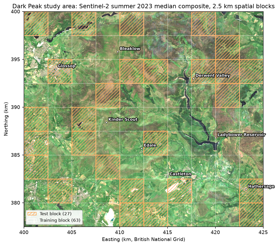
The study area is a 25 × 22.5 km rectangle of the Dark Peak, on the British National Grid (EPSG:27700) at 10 m. It covers the peat plateaux of Kinder Scout and Bleaklow, the Edale and Hope valleys, the edge of Glossop and the Derwent and Ladybower reservoirs. If you followed Monitoring reservoir water quality with Sentinel-2, you have already seen these reservoirs.
The labels come from Living England 2022-23, Natural England’s broad habitat map, published under the Open Government Licence. It is reachable from a public ArcGIS service with no login. Each polygon has a primary habitat and a reliability rating from Very Low to Very High. We map its habitats to nine classes:
| id | Class | Living England habitats | Share of area |
|---|---|---|---|
| 1 | Blanket bog | Bog | 16.1% |
| 2 | Heath | Dwarf Shrub Heath | 26.9% |
| 3 | Bracken | Bracken | 7.4% |
| 4 | Semi-natural grassland | Unimproved Grassland | 17.1% |
| 5 | Improved grassland | Improved and Semi-Improved Grassland; Arable and Horticultural | 16.0% |
| 6 | Broadleaf woodland | Broadleaved, Mixed and Yew Woodland; Scrub | 7.1% |
| 7 | Conifer woodland | Coniferous Woodland | 3.1% |
| 8 | Water | Water | 1.5% |
| 9 | Built-up and bare | Built-up Areas and Gardens; Bare Ground; Bare Sand | 4.6% |
Semi-natural grassland is mostly acid grassland on the gritstone, but it is calcareous grassland on the limestone south of Castleton. Living England does not separate the two. Fen, marsh and swamp covers only about 2 km² and is left out.
The series’ shared script prepare_data.py downloads the polygons, rasterises them onto the grid and draws the samples. It takes 1,000 “pure” pixels per class from High or Very High reliability polygons, where all eight neighbours share the class. Then it cuts the area into 90 blocks of 2.5 km and assigns 27 blocks (30%) to the test set with a fixed seed. Samples within 50 m of a block edge are dropped, so no test pixel touches a training block. The result is committed to the repository as a small CSV, so every part of the series trains and tests on exactly the same points.
import habitat_common as hc                      # the series' shared module
labels = hc.label_raster() # Living England 2022-23 on the 10 m grid (0 = unlabelled)samples = hc.load_samples() # the committed sample design, with split and foldblocks = hc.load_blocks()AOI: Dark Peak (Kinder Scout, Bleaklow, Edale and the Hope Valley)grid: EPSG:27700, 10 m, bounds (400000, 377500, 425000, 400000), 2500 x 2250 pixels9,000 samples in 90 blocks of 2.5 km; 6,544 train / 2,456 test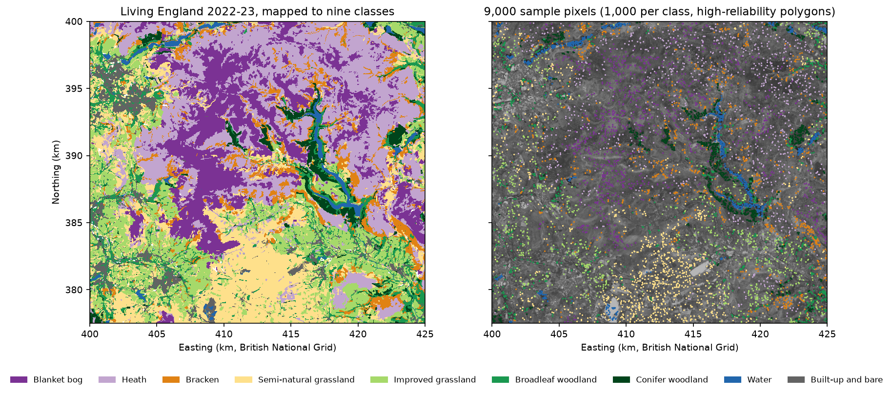
Step 1: seasonal Sentinel-2 composites
Habitats differ most in when they are green. Bracken is brown until late May and then lush; improved pasture is green from early spring; bog stays pale all year. So we build four seasonal composites for 2023, the year of the labels, rather than one summer image.
The shared module searches the Planetary Computer for every Sentinel-2 L2A scene over the area. It removes duplicate processing baselines and masks cloud and shadow with the scene classification layer (SCL), growing the cloud mask by 20 m. It keeps dates with at least 5% of the area clear and takes the per-pixel median reflectance. Sentinel-2 cloud masking in Python compares SCL with better cloud masks, and NDVI time series with odc-stac explains the loading pattern.
dates = hc.s2_dates() # clear fraction of each usable 2023 dateS = hc.s2_seasonal_composites() # {"winter", "spring", "summer", "autumn"} -> Datasetfor season, ds in S.items(): n = ds["n_clear"].values print(f"{season:<7} median {np.median(n):.0f} clear views; none at {(n == 0).mean():.2%} of pixels")50 dates with at least 5% of the AOI clear; median clear fraction 31%winter median 3 clear views; none at 3.56% of pixelsspring median 5 clear views; none at 0.02% of pixelssummer median 7 clear views; none at 0.03% of pixelsautumn median 6 clear views; none at 0.00% of pixelsThe Pennines are cloudy. Of the 73 Sentinel-2 dates in 2023 with less than 90% scene cloud, only 50 were at least 5% clear over the study area, and the median usable date was only 31% clear. A typical pixel has just three clear winter views and seven in summer. That is enough for a median, but not for a dense time series; Part 4 deals with the gaps.
Step 2: spectral indices for upland habitats
From the composites we compute a few indices per season, plus single bands. Each index targets a property that differs between habitats:
- NDVI, (NIR − red) / (NIR + red): greenness. High for improved grass, low for bare peat and water.
- NDMI, (NIR − SWIR) / (NIR + SWIR): moisture in leaves and soil. Grassland is far moister in spectral terms than moorland in spring.
- NDWI, (green − NIR) / (green + NIR): open water.
- dNDVI, summer NDVI minus spring NDVI: the late green-up of bracken and deciduous woodland.
def nd(a, b):    with np.errstate(divide="ignore", invalid="ignore"):        return (a - b) / (a + b)

def features(S):    """Index and band layers used by the rules: 2-D float32 arrays on the shared grid."""    f = {}    for s, ds in S.items():        b = {k: ds[k].values for k in hc.S2_BANDS}        f[f"ndvi_{s}"] = nd(b["B08"], b["B04"])     # greenness        f[f"ndmi_{s}"] = nd(b["B08"], b["B11"])     # canopy and soil moisture        f[f"ndwi_{s}"] = nd(b["B03"], b["B08"])     # open water (McFeeters)        f[f"nir_{s}"], f[f"red_{s}"] = b["B08"], b["B04"]        f[f"swir_{s}"], f[f"swir2_{s}"] = b["B11"], b["B12"]    f["dndvi_spring_summer"] = f["ndvi_summer"] - f["ndvi_spring"]   # late green-up    return f
Before writing any rules, look at the medians of each feature by class in the training samples:
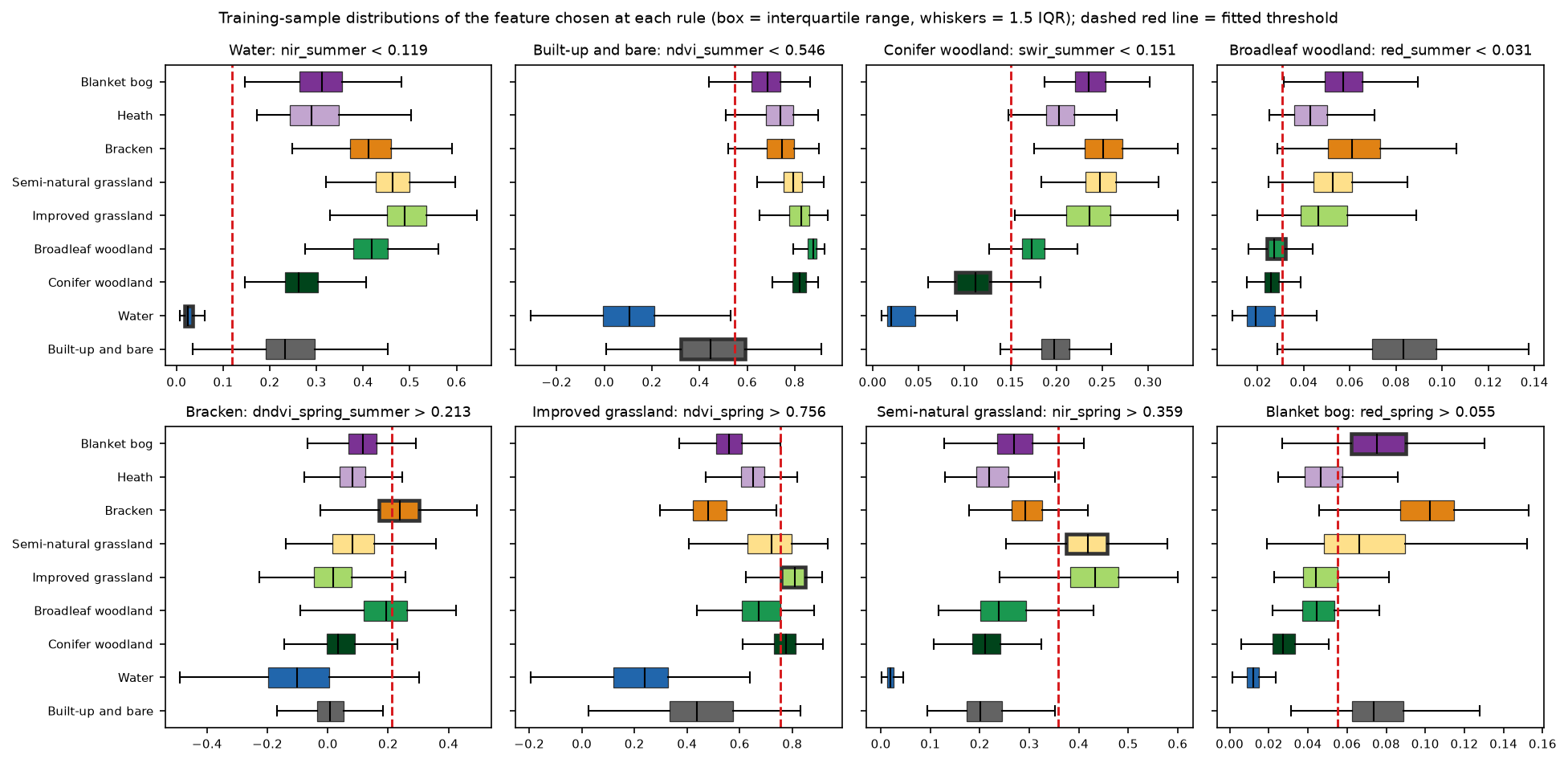
bog heath brack semin impro broad conif water builtndvi_spring 0.559 0.650 0.481 0.722 0.810 0.674 0.775 0.238 0.438ndvi_summer 0.686 0.741 0.746 0.793 0.828 0.877 0.822 0.107 0.447dndvi_spring_summer 0.116 0.082 0.240 0.082 0.019 0.194 0.034 -0.101 0.006ndmi_spring 0.071 0.061 -0.011 0.242 0.325 0.134 0.345 0.022 0.053nir_summer 0.311 0.289 0.411 0.463 0.488 0.418 0.261 0.024 0.233swir_summer 0.236 0.203 0.251 0.248 0.236 0.173 0.112 0.020 0.198red_summer 0.057 0.043 0.061 0.053 0.046 0.027 0.026 0.019 0.083red_spring 0.075 0.047 0.102 0.066 0.044 0.044 0.027 0.012 0.074Some classes stand out. Water has almost no near-infrared reflectance (0.024). Conifers are dark in the shortwave infrared (0.112). Bracken has the biggest jump in NDVI from spring to summer (0.240). Others overlap badly. Bog and heath differ by only a few hundredths in most features: heath is a little darker in red, and bog is paler in spring, where cotton-grass and bare peat show through. Semi-natural and improved grassland differ mainly in how green they are in spring.
Step 3: a decision list with thresholds fitted from data
A decision list peels off one class at a time, starting with the easiest. Each pixel takes the first rule it satisfies, and whatever is left becomes heath, the most common class. We fix the order and a short list of candidate features for each class from the ecology. The training samples then choose the feature and threshold that give the best F1 score for that class among the samples still unclassified at that point.
NODES = [    ("water", ["nir_summer", "ndwi_summer"]),             # absorbs near-infrared    ("built_bare", ["ndvi_summer", "ndvi_spring"]),       # little or no vegetation    ("conifer", ["swir_summer", "swir2_summer"]),         # dark, shaded evergreen    ("broadleaf", ["red_summer", "ndmi_summer", "ndvi_summer", "swir2_summer"]),    ("bracken", ["dndvi_spring_summer", "ndvi_spring"]),  # brown spring, lush summer    ("improved_grass", ["ndvi_spring", "nir_spring", "ndmi_spring", "ndvi_winter"]),    ("seminat_grass", ["ndmi_spring", "nir_spring", "ndvi_spring"]),    ("bog", ["red_spring", "ndvi_spring", "nir_summer"]), # pale cotton-grass, bare peat]DEFAULT = "heath"   # whatever is left: dark dwarf-shrub heath

def best_threshold(x, pos):    """Threshold and direction that maximise F1 for 'pos' against everything else."""    ok = ~np.isnan(x)    x, pos = x[ok], pos[ok]    best = (-1.0, np.nan, "<")    for sign, op in ((1, "<"), (-1, ">")):        v = sign * x        o = np.argsort(v, kind="stable")        vs, p = v[o], pos[o]        tp, fp = np.cumsum(p), np.cumsum(~p)        f1 = 2 * tp / (tp + fp + p.sum())        f1[:-1][np.diff(vs) == 0] = -1          # only cut between distinct values        i = int(np.argmax(f1[:-1]))        if f1[i] > best[0]:            best = (float(f1[i]), float(sign * (vs[i] + vs[i + 1]) / 2), op)    return best
fit_rules walks down the list, keeps the best candidate at each node and removes the samples it captures. It sees only the 63 training blocks:
1. Water if nir_summer < 0.119 (train F1 0.94, n = 6,544)2. Built-up and bare if ndvi_summer < 0.546 (train F1 0.68, n = 5,791)3. Conifer woodland if swir_summer < 0.151 (train F1 0.94, n = 5,142)4. Broadleaf woodland if red_summer < 0.031 (train F1 0.75, n = 4,251)5. Bracken if dndvi_spring_summer > 0.213 (train F1 0.65, n = 3,694)6. Improved grassland if ndvi_spring > 0.756 (train F1 0.69, n = 3,020)7. Semi-natural grassland if nir_spring > 0.359 (train F1 0.68, n = 2,207)8. Blanket bog if red_spring > 0.055 (train F1 0.62, n = 1,763)9. otherwise -> HeathEvery rule is a single comparison you can read and check against the ecology. The figure below shows why some are clean and some are not. The water and conifer thresholds sit in clear gaps between classes. The bog threshold cuts through the middle of overlapping boxes.
Step 4: classify the whole study area
Applying the list to every pixel is a few lines of NumPy, and the map is saved as a GeoTIFF on the shared grid:
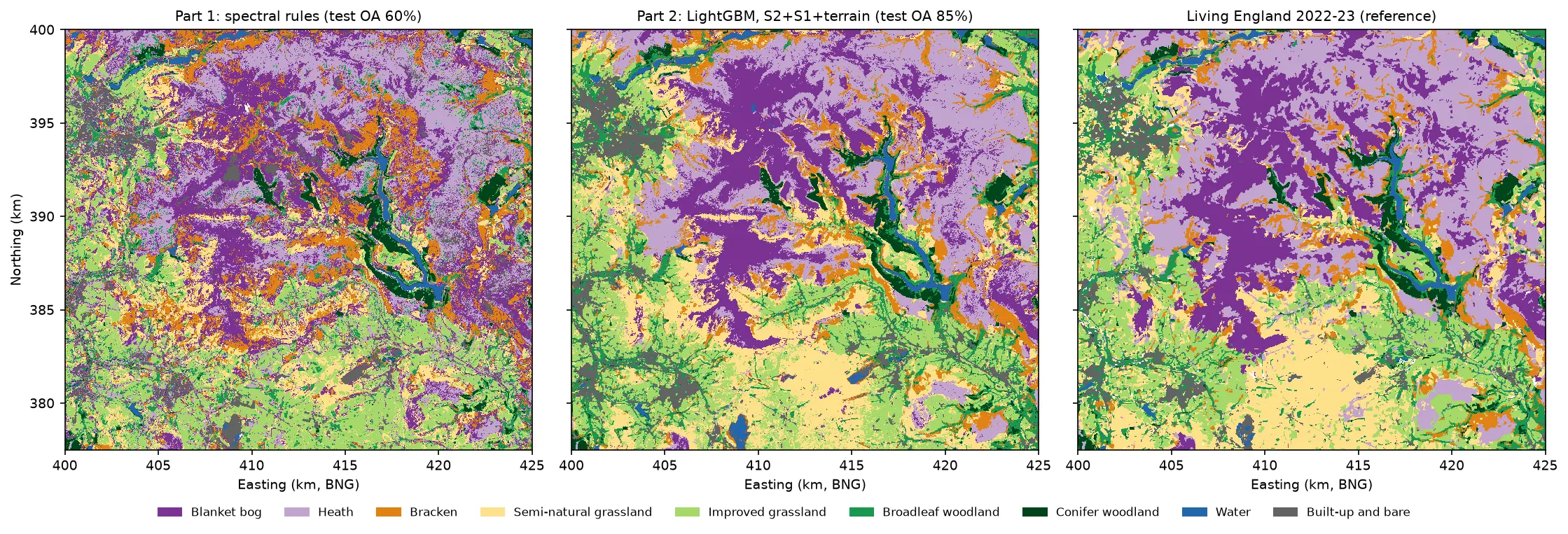
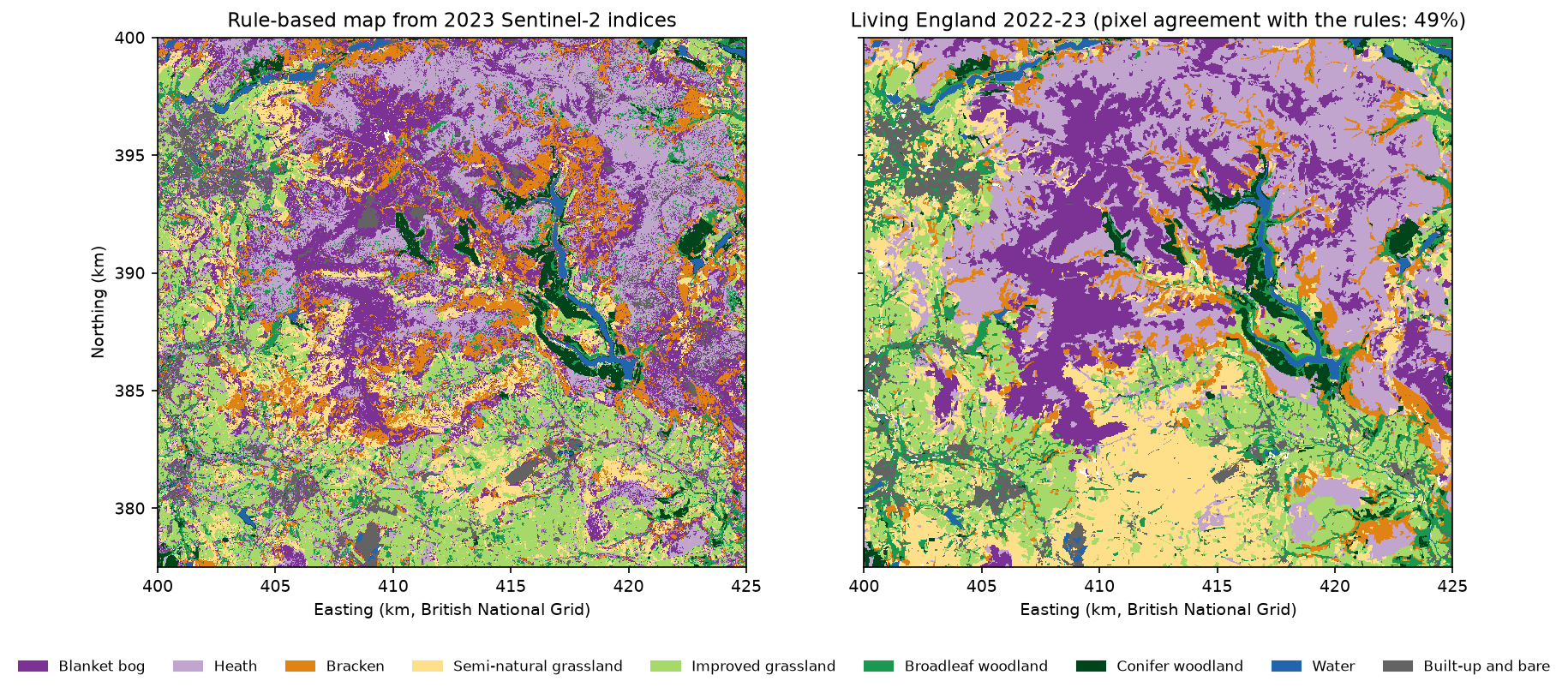
pred_key = apply_rules(rules, lambda f: FEAT[f])pred = np.zeros(hc.shape(), "uint8")for k in KEYS: pred[pred_key == k] = KEY_ID[k]nodata = np.isnan(FEAT["ndvi_summer"]) | np.isnan(FEAT["ndvi_spring"])pred[nodata] = 0hc.write_geotiff(OUT / "habitat_rules_2023.tif", pred, nodata=0) rules_km2 living_england_km2Blanket bog 131.0 90.5Heath 109.9 151.5Bracken 64.1 41.6Semi-natural grassland 63.5 96.1Improved grassland 101.9 90.0Broadleaf woodland 35.4 39.7Conifer woodland 17.3 17.2Water 6.3 8.4Built-up and bare 32.9 25.7unclassified (no clear spring or summer view): 0.05% of pixelsThe rules get the big picture right: bog and heath on the plateaux, bracken on the valley sides, grass and woodland below. Conifer area matches Living England almost exactly. But the rules map 45% more bog and 28% less heath than Living England, and a third less semi-natural grassland.
Step 5: accuracy assessment on the test blocks
Now the main event. We apply the same rules to the 2,456 samples in the 27 test blocks and compare them with their Living England labels in a confusion matrix. Rows are the reference, and columns are the map.
bog heath brack semin impro broad conif water builtref bog 170 28 24 5 1 0 0 0 29ref heath 58 197 13 5 5 27 1 0 20ref bracken 77 10 172 13 1 2 0 0 10ref seminat_grass 24 6 9 84 228 13 0 0 6ref improved_grass 5 13 4 28 210 15 0 0 7ref broadleaf 10 35 22 5 34 188 22 0 0ref conifer 3 8 0 2 2 6 99 0 0ref water 3 3 1 0 0 0 3 115 13ref built_bare 68 33 0 1 13 3 1 5 238From the matrix come two per-class measures:
- Producer’s accuracy (recall) is the diagonal divided by the row total. It answers “of the real bog, how much did the map find?”
- User’s accuracy (precision) is the diagonal divided by the column total. It answers “if I visit a pixel the map calls bog, how likely is it to be bog?”
pa = np.diag(m) / m.sum(1) # producer's accuracy (recall): rows are referenceua = np.diag(m) / np.where(m.sum(0) == 0, np.nan, m.sum(0)) # user's accuracy (precision)f1 = 2 * pa * ua / (pa + ua) n_test producers_acc users_acc f1Blanket bog 257 0.661 0.407 0.504Heath 326 0.604 0.592 0.598Bracken 285 0.604 0.702 0.649Semi-natural grassland 370 0.227 0.587 0.327Improved grassland 282 0.745 0.425 0.541Broadleaf woodland 316 0.595 0.740 0.660Conifer woodland 120 0.825 0.786 0.805Water 138 0.833 0.958 0.891Built-up and bare 362 0.657 0.737 0.695overall accuracy 0.600 (n = 2,456 samples in 27 test blocks) 95% CI treating samples as independent: 0.580 to 0.619 95% CI from a block bootstrap: 0.527 to 0.664macro F1 0.630; Cohen's kappa 0.547disagreement 0.400 = quantity 0.157 + allocation 0.243area-weighted agreement (sum of reference-area share x producer's accuracy): 0.583wall-to-wall agreement with Living England over all 1,680,440 labelled test-block pixels: 0.483wall-to-wall agreement over the whole study area (train and test blocks): 0.490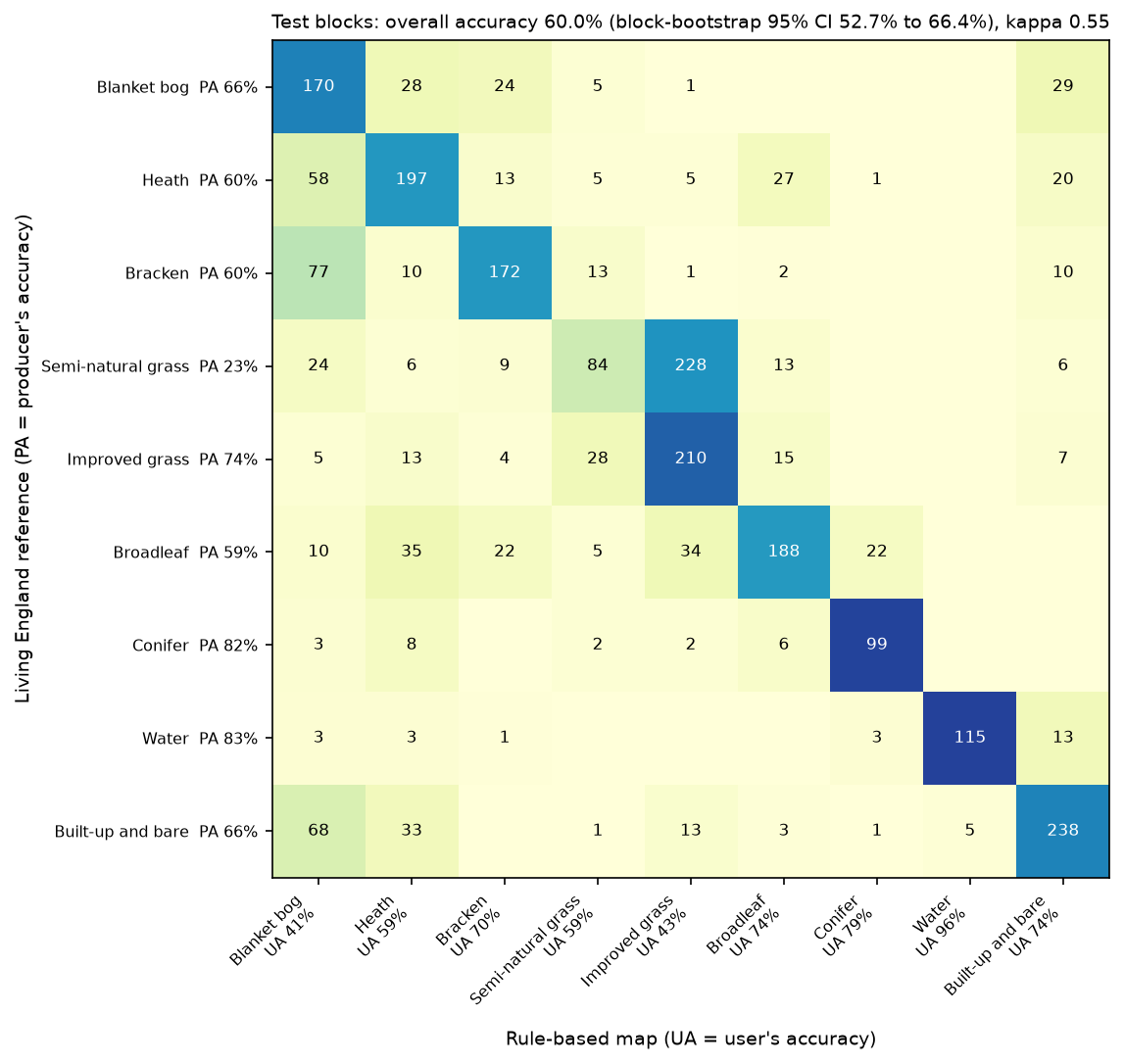
How to read it:
- The two measures tell different stories. Blanket bog has a producer’s accuracy of 66% but a user’s accuracy of only 41%. The map finds most bog, but it also calls 77 bracken samples and 68 built-up or bare samples bog. On these moors, “bare” is mostly eroded peat, so this is partly a label boundary problem, not just a spectral one.
- Semi-natural grassland is the weak spot. 228 of 370 test samples were mapped as improved grassland, so its producer’s accuracy is 23%. Nine in ten of them are in the south of the area, mostly limestone grassland around Castleton, which is as green in spring as fertilised pasture. A single spring greenness threshold cannot separate them; Part 2 adds the full seasonal profile and radar.
- Bog versus heath is the hardest ecological split. 58 heath samples were mapped as bog and 28 bog samples as heath. Both are dark peat with low vegetation. Part 2 makes this its case study.
Overall accuracy and an honest confidence interval
Overall accuracy (OA) is the diagonal total over all samples: 0.600. The textbook 95% interval, ±1.96 × √(OA × (1 − OA) / n), gives 58.0% to 61.9%. That formula assumes every sample is independent, but our samples come in clusters inside 27 blocks, and samples in the same block share their errors. So we resample whole blocks instead, 2,000 times:
for _ in range(2000): # resample whole test blocks, not pixels pick = rng.choice(ub, ub.size, replace=True) idx = np.concatenate([np.flatnonzero(tb == b) for b in pick]) boot.append(correct[idx].mean())lo, hi = np.percentile(boot, [2.5, 97.5])The block bootstrap gives 52.7% to 66.4%, more than three times as wide. That is the honest uncertainty, and it matters for this series: a later method that scores 62% has not clearly beaten 60%. The five-fold blocked cross-validation on the training blocks tells the same story, with fold accuracies from 62.9% to 72.0%:
fold OA: 0.693, 0.697, 0.629, 0.720, 0.681; mean 0.684 +/- 0.030Kappa, and why not to lean on it
Cohen’s kappa is 0.547. Kappa compares OA with the agreement expected by chance from the row and column totals. It is widely reported, but Pontius and Millones (2011) showed that it adds little. Its “chance” baseline is not a sensible alternative map, it is not a probability, and it mixes up two very different kinds of error. They recommend splitting the 40% disagreement instead:
- Quantity disagreement (15.7%): the map has the wrong amount of some classes, such as too much bog and too little semi-natural grassland.
- Allocation disagreement (24.3%): the amounts are right, but in the wrong places.
Report kappa if a reviewer or a specification asks for it, but interpret the confusion matrix, the per-class accuracies and these two components.
Sample accuracy is not map accuracy
Three more numbers show what the 60% does not mean:
- The sample is balanced, with 1,000 per class, but the landscape is not: heath covers 27% of the area and water 1.5%. Weighting each class’s producer’s accuracy by its share of the area gives 58.3%. Part 5 does this properly, with an area-adjusted estimator and confidence intervals (Olofsson et al. 2014).
- The samples are pure pixels from reliable polygons. Over every labelled pixel in the test blocks, including edges, mixtures and low-reliability polygons, the map agrees with Living England on only 48.3%. Most of the gap is on boundaries and in mosaics that no pixel classifier will match exactly.
- All of it is agreement with another model, not with field data.
Step 6: why a random split overstates accuracy
Most tutorials split samples into training and test sets at random. Here that means a test pixel is usually a stone’s throw from a training pixel in the same field or the same patch of moor. Spatial autocorrelation makes neighbours similar, so the test is easy. We measure the distance from each test sample to its nearest training sample under both designs:
median distance from test to nearest training sample: random split 103 m, block split 785 mTo see what that does to accuracy, we repeat 20 random 70/30 splits of the 9,000 samples, and 20 splits of the 90 blocks. We refit the rules each time. We also add a deliberately silly classifier that ignores the imagery and copies the label of the nearest training sample, using only its coordinates:
def nn_coords(tr_idx, te_idx): """A 'model' that sees only location: the label of the nearest training sample.""" j = cKDTree(xy[tr_idx]).query(xy[te_idx])[1] return (X["cls"].to_numpy()[tr_idx][j] == X["cls"].to_numpy()[te_idx]).mean()overall accuracy over 20 repeated 70/30 splits: rules nearest_neighbour_xy mean std mean stdsplitblocks 0.643 0.029 0.412 0.049random 0.670 0.010 0.806 0.005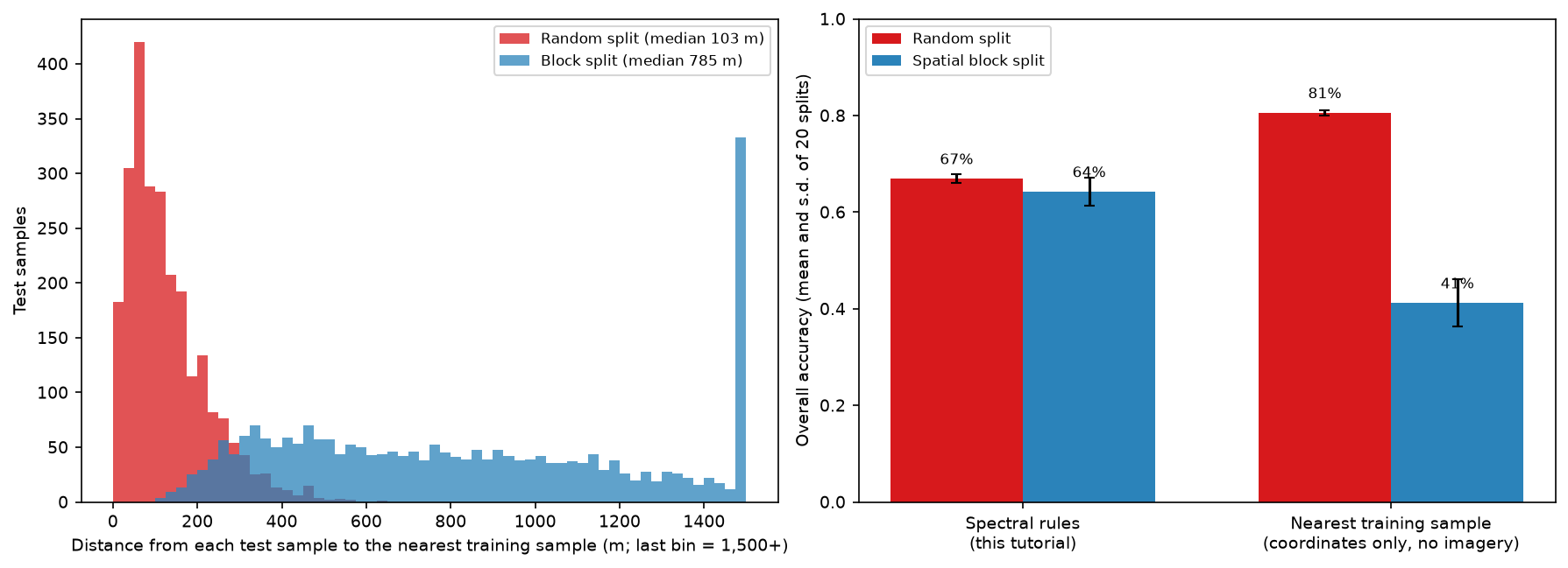
The coordinates-only model, which has never seen a satellite image, scores 81% with a random split. That beats our spectral rules. With a block split it falls to 41%. A random split mostly rewards memorising where each habitat is, not recognising it.
Our eight rules are barely affected (67% against 64%), because eight thresholds are too few to memorise anything. Flexible models are another matter. A random forest or a neural network can learn the fine detail of where each sample sits, and the gap grows with the model’s capacity. That is why every part of this series uses the same block split, and why you should treat any random-split accuracy for a habitat map with suspicion. Land cover classification with a Sentinel-2 random forest shows the same effect for a random forest.
The baseline for this series
| Measure (test blocks, n = 2,456) | Part 1: spectral rules |
|---|---|
| Overall accuracy | 0.600 (block-bootstrap 95% CI 0.527 to 0.664) |
| Macro F1 | 0.630 |
| Cohen’s kappa | 0.547 |
| Blocked 5-fold CV on training blocks | 0.684 ± 0.030 |
| Wall-to-wall agreement, test blocks | 0.483 |
| Hardest classes (F1) | Semi-natural grassland 0.33, blanket bog 0.50 |
Every later part reports the same measures on the same 2,456 test samples, so the gains can be read straight from this table.
How the series beats this baseline
| Part | Method | OA (95% CI) | Macro F1 |
|---|---|---|---|
| 1 | Spectral rules (this tutorial) | 0.600 (0.527–0.664) | 0.630 |
| 2 | LightGBM on Sentinel-2, Sentinel-1 and terrain | 0.853 (0.801–0.892) | 0.862 |
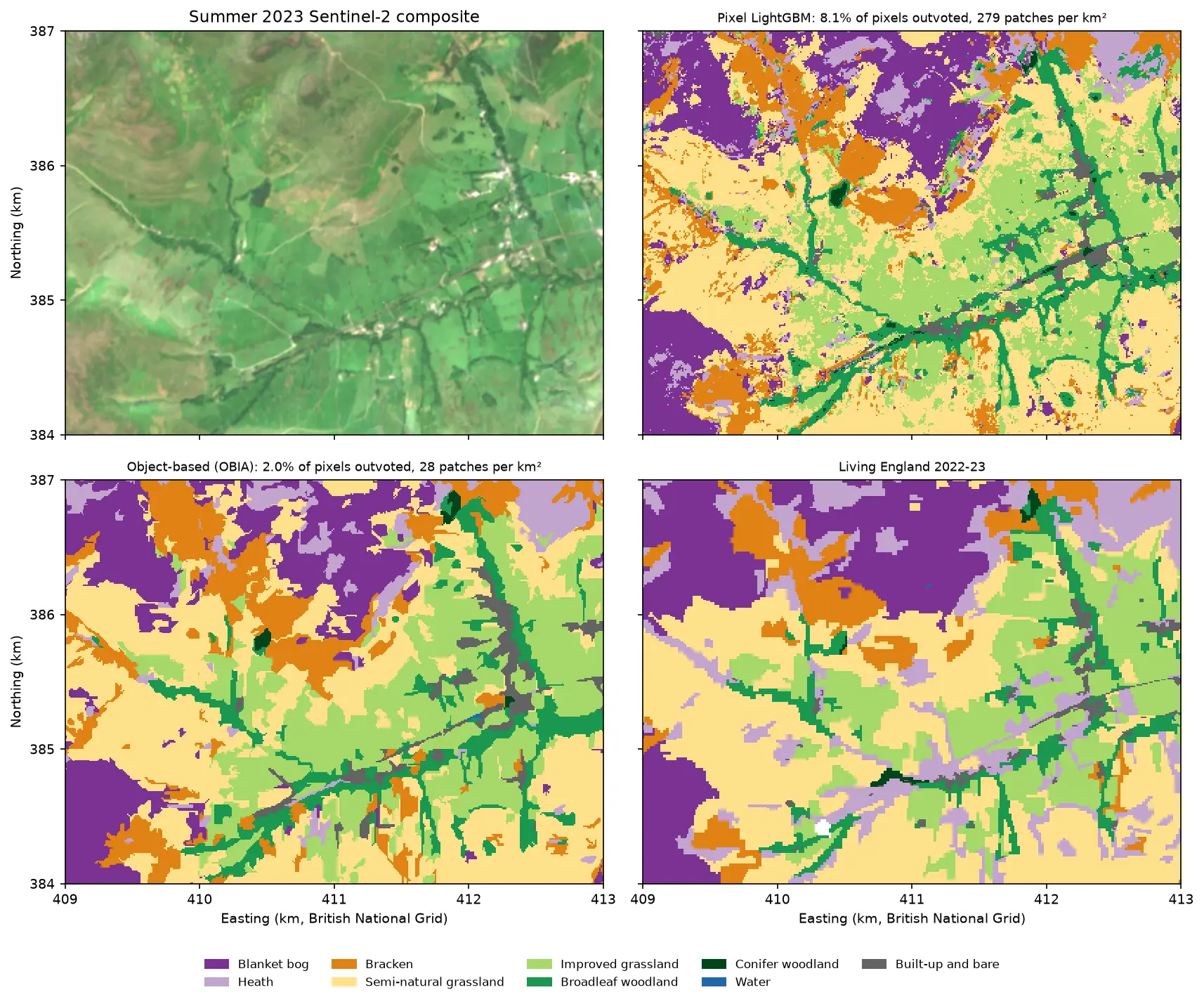
| 3 | Object-based LightGBM (OBIA), Sentinel-2 only | 0.794 (0.729–0.845) | 0.808 |
| 4 | TempCNN on the Sentinel-2 time series | 0.851 (0.811–0.884) | 0.858 |
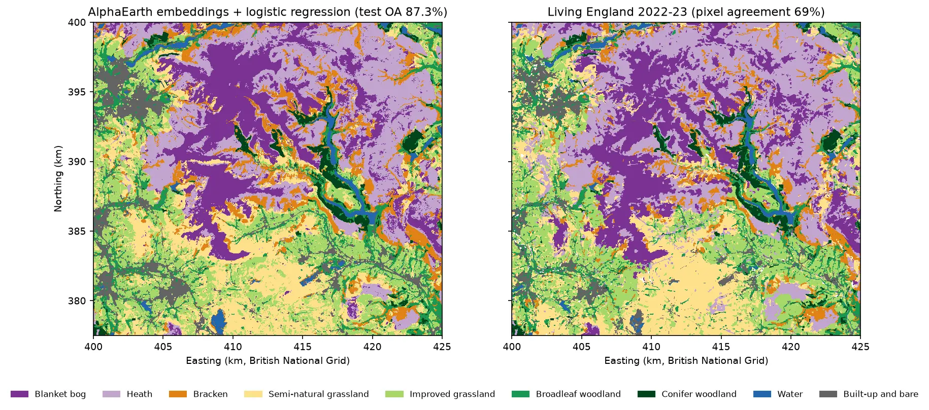
| 5 | AlphaEarth embeddings + logistic regression | 0.873 (0.841–0.902) | 0.878 |
Every later method beats the rules by 19 to 27 points, far outside the block-bootstrap uncertainty, and bog and semi-natural grassland improve the most. The differences between Parts 2, 4 and 5 are within the uncertainty. What sets the embeddings apart is that they need far fewer labels. The full comparison in Part 5 adds kappa, wall-to-wall agreement, runtimes and the map-noise and area-adjusted results.
Limitations
- The labels are a model. Living England is a classification with its own errors, and its bare ground on the moors is often eroded peat that ecologists would call degraded bog. Our “errors” include its errors.
- One year, one area. The thresholds are fitted to 2023 in the Dark Peak. A wetter spring, a different processing baseline or a lowland landscape would move them. Refit on local samples before using the rules elsewhere.
- Clouds. A typical pixel has only three clear winter views, and 3.6% of pixels have none. The rules use only spring and summer features, so only 0.05% of the map is unclassified, but noisy medians cause speckle.
- Pixels, not patches. The map is noisy at pixel scale, which hurts wall-to-wall agreement. Part 3 classifies image objects instead.
- Balanced, pure samples. Sample accuracy flatters the map. Use area-weighted estimates (Part 5) to report the accuracy of a map product.
Frequently asked questions
Can Sentinel-2 map habitats?
Yes, at broad habitat level. Natural England’s Living England map is itself made from Sentinel-1 and Sentinel-2. At 10 m, Sentinel-2 reliably separates water, woodland, conifers, built-up land and improved grassland. Upland habitats such as blanket bog, heath and rough grassland are harder, because their spectra overlap. Seasonal composites help a lot, and radar and machine learning help further.
Which spectral indices are best for habitat mapping?
There is no single best index. NDVI captures greenness, NDMI captures moisture and separates grassland from moorland, and NDWI or near-infrared reflectance finds water. Shortwave infrared separates conifers, and the change in NDVI between spring and summer picks out bracken. The season often matters more than the index: compute each index for several seasons and let the training data choose.
What is the difference between user’s and producer’s accuracy?
Producer’s accuracy is the share of reference samples of a class that the map gets right (recall): it measures omission. User’s accuracy is the share of pixels mapped as a class that are right (precision): it measures commission. A map can find most of a class (high producer’s) while over-mapping it (low user’s), as our blanket bog does with 66% and 41%.
Should I report the kappa coefficient?
Report it if a client, a journal or a specification requires it, but do not rely on it. Kappa compares the map with a “chance” agreement that is not a meaningful alternative, and it does not say what went wrong. A confusion matrix, per-class user’s and producer’s accuracy, and overall accuracy with a confidence interval tell readers more. Splitting the disagreement into quantity and allocation, as Pontius and Millones (2011) suggest, shows what kind of error the map makes.
Why is my random train/test split accuracy so high?
Because test samples are next to training samples. Neighbouring pixels are similar (spatial autocorrelation), so a random split mostly tests interpolation. In our data, a model that only copies the label of the nearest training sample scores 81% with a random split and 41% with a spatial block split. Use spatial blocks or regions for testing, and report the uncertainty by resampling whole blocks.
Where can I get free habitat labels for England?
The Living England Habitat Map from Natural England covers all of England and is free under the Open Government Licence, with no login. The Priority Habitat Inventory maps priority habitats in more detail but is not wall-to-wall. The UKCEH Land Cover Map is widely used but needs a licence or a login for the full product. For anything important, add your own field or photo-interpreted samples.
Next steps
- Load and composite Sentinel-2 in more depth with NDVI time series with odc-stac, and improve the cloud mask with Sentinel-2 cloud masking in Python.
- Summarise the habitat map by moorland unit or catchment with zonal statistics in Python.
- See a supervised alternative on global labels in Land cover classification with a Sentinel-2 random forest.
- Continue the series: Part 2 adds Sentinel-1 radar and terrain to LightGBM, Part 3 classifies image objects, Part 4 trains a temporal neural network in PyTorch, and Part 5 uses AlphaEarth foundation-model embeddings with few labels.
- Prepare for the radar features of Part 2 with SAR speckle filtering in Python.
- For deep learning on image chips rather than pixel time series, start with training data for deep learning on satellite imagery, then train a U-Net and run it over large rasters. For segmentation of very high resolution imagery, see Segment Anything on satellite imagery.
Data and licences
- Living England Habitat Map 2022-23: © Natural England, under the Open Government Licence v3.0. Contains Ordnance Survey data © Crown copyright and database right. Accessed from Natural England’s public ArcGIS service on 21 October 2026.
- Sentinel-2 L2A: contains modified Copernicus Sentinel data 2023, free and open under the Copernicus data licence. Accessed from the Microsoft Planetary Computer.
- References: Pontius, R. G. and Millones, M. (2011), “Death to Kappa: birth of quantity disagreement and allocation disagreement for accuracy assessment”, International Journal of Remote Sensing 32(15), 4407–4429. Olofsson, P. et al. (2014), “Good practices for estimating area and assessing accuracy of land change”, Remote Sensing of Environment 148, 42–57.
- Code:
habitat_rules.pyand the shared series module (habitat_common.py,prepare_data.py, sample CSVs), tested with Python 3.12.0, odc-stac 0.5.3, pystac-client 0.9.1, rasterio 1.5.2, geopandas 1.2.0, pandas 3.0.6 and matplotlib 3.11.2.
Key terms
- Habitat map
- A map of vegetation and land types defined by ecological criteria, such as blanket bog or dwarf shrub heath, rather than by land use or simple land cover.
- Spectral index
- A formula that combines two or more image bands to highlight one property, such as greenness (NDVI) or moisture (NDMI). Normalised differences, (a − b) / (a + b), are the most common form.
- Decision list
- An ordered set of if-then rules. Each pixel takes the class of the first rule it satisfies, and pixels that satisfy no rule get a default class.
- Producer's accuracy
- For one class, the share of reference samples of that class that the map labels correctly (recall). Low producer's accuracy means the map misses the class.
- User's accuracy
- For one class, the share of map pixels labelled as that class that are correct (precision). Low user's accuracy means the class is over-mapped.
- Spatial autocorrelation
- The tendency of nearby places to be similar. It makes test samples next to training samples easy, so random train/test splits overstate accuracy.
Data for this tutorial
- Living England Habitat Map · Natural England's broad habitat map, used as labels (2022-23 release)
- Microsoft Planetary Computer · Sentinel-2 L2A through STAC, no account needed
Licences and formats for each source are listed in the GIS data sources catalogue.