SAR speckle filtering in Python: Lee, refined Lee, Frost and Gamma-MAP on Sentinel-1

Short answer: a speckle filter in Python needs only NumPy and SciPy. Compute the local mean and variance with scipy.ndimage.uniform_filter, then blend each pixel towards the local mean according to how much of the local variance is explained by speckle alone. That is the Lee filter: out = mean + k * (img - mean), with k = var_x / var and var_x = (var - mean² / ENL) / (1 + 1 / ENL). Always filter the linear backscatter (power), not decibels, and convert to dB afterwards. For Sentinel-1, a 7 × 7 Lee or Gamma-MAP filter is a good default.

Every radar image is grainy. That grain, speckle, is not dirt on the lens. It is physics: each pixel contains many small scatterers whose echoes add up with random phases, so neighbouring pixels of the same field come out bright, dark or anywhere in between. Speckle makes thresholds noisy, classifiers confused and maps ugly, so almost every SAR workflow starts with a speckle filter.

In this tutorial we write the six classic filters ourselves and test them on real Sentinel-1 data over Rutland Water in the East Midlands, a 13 × 11 km area with a reservoir, lagoons, the town of Oakham, woods and large arable fields. You will learn how to:

1. stream a stack of Sentinel-1 RTC chips from the Planetary Computer;
2. test the multiplicative speckle model against the gamma distribution, and see why dB averaging is biased;
3. implement boxcar, Lee, refined Lee, enhanced Lee, Frost and Gamma-MAP filters in NumPy and SciPy;
4. score them with the equivalent number of looks (ENL), an edge-preservation index (EPI), the ratio image and runtime, using a 29-date average as a speckle-free reference.

All outputs below are real results from speckle_filters.py, run on 21 October 2026 with Python 3.12, NumPy 2.5.4 and SciPy 1.18.1.

Step 1: read a stack of Sentinel-1 chips

We search the Planetary Computer’s sentinel-1-rtc collection for one relative orbit, so every date has the same viewing geometry, and read a small window of the VV band from each Cloud Optimised GeoTIFF:

BBOX = (-0.76, 52.61, -0.56, 52.71)   # lon/lat: Rutland Water, Oakham and farmland, East Midlands, England
ORBIT = 154                           # one relative orbit (descending): identical geometry on every date
SEASON = "2025-10-01/2026-03-31"
TARGET = "2026-01-10"                 # the single date we filter

catalog = pystac_client.Client.open("https://planetarycomputer.microsoft.com/api/stac/v1",
                                    modifier=planetary_computer.sign_inplace)
items = sorted(catalog.search(collections=["sentinel-1-rtc"], bbox=BBOX, datetime=SEASON,
                              query={"sat:relative_orbit": {"eq": ORBIT}}).items(), key=lambda i: i.datetime)
to_utm = Transformer.from_crs(4326, items[0].properties["proj:code"], always_xy=True)
xs, ys = to_utm.transform([BBOX[0], BBOX[2]], [BBOX[1], BBOX[3]])


def read_vv(item):
    """Read the chip of linear gamma0 VV at the native 10 m grid (only the needed COG tiles are fetched)."""
    with rasterio.open(item.assets["vv"].href) as src:
        win = from_bounds(xs[0], ys[0], xs[1], ys[1], src.transform).round_offsets().round_lengths()
        a = src.read(1, window=win).astype("float32")
        a[a == src.nodata] = np.nan
    return a


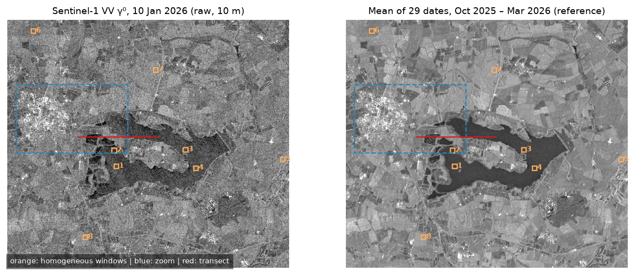
stack = np.stack([read_vv(i) for i in items])
img = stack[[i.id for i in items].index(target.id)]
ref = np.nanmean(stack, axis=0)        # multi-temporal multilook: nearly speckle-free, edges kept

29 scenes from relative orbit 154, 06 Oct 2025 to 29 Mar 2026
target: S1A_IW_GRDH_1SDV_20260110T062247_20260110T062312_062701_07DC9E_rtc | sentinel-1a | looks 5 x 1 | nominal ENL 4.4 | EPSG:32630
read 29 chips of 1156 x 1316 pixels (10 m) in 20 s; NaN pixels in target: 0
target gamma0 VV: min 0.0018, median 0.0980, max 111.50 (linear)

With Sentinel-1A and Sentinel-1C both flying, this orbit is revisited every 6 days, which gives 29 dates in six months. We filter one of them, 10 January 2026. The mean of all 29 dates is our reference. Averaging 29 independent images cuts speckle variance about 29-fold without blurring a single edge, as long as the landscape does not change much. It is the closest thing to a speckle-free “truth” that we can get for free.

The values are linear gamma-nought (γ⁰), a ratio of powers. Note the range: from 0.0018 (−27 dB, calm water) to 111 (+20 dB, a metal roof facing the radar). Speckle filters work on these numbers.

Step 2: the multiplicative speckle model

Over a uniform area, the measured intensity I is the true backscatter R multiplied by a random speckle term n:

I = R · n, with mean of n = 1 and variance of n = 1/L

where L is the number of looks. For fully developed speckle in an image averaged over L independent looks, n follows a gamma distribution with shape L and scale 1/L. A single look gives an exponential distribution, the noisiest case (L = 1). Two things follow:

• Speckle is signal-dependent. Its standard deviation grows with the backscatter, so bright fields look noisier than dark water in absolute terms. Additive-noise filters, such as a Gaussian blur tuned to a fixed noise level, do not fit.
• The coefficient of variation (standard deviation ÷ mean) of pure speckle is a constant, 1/√L. Any area with a higher CV contains real structure, such as an edge or a point target. That is the test that every adaptive filter below uses.

To check this on real data, we need uniform areas. We let the reference image choose them: the code slides a 21 × 21 pixel (210 m) window over the 29-date mean and picks the four windows with the lowest CV on water and four on land. The ENL of each window is mean² / variance of the single-date image:

def enl(x, kind=None):
    """Equivalent number of looks: mean^2 / variance of intensity, averaged over the homogeneous windows."""
    return float(np.mean([np.nanmean(x[s]) ** 2 / np.nanvar(x[s]) for s, k in zip(sl, kinds) if kind in (None, k)]))


norm = np.concatenate([(img[s] / np.nanmean(img[s])).ravel() for s in sl])   # speckle samples, mean 1
L_fit, _, _ = stats.gamma.fit(norm, floc=0)

window 1 (water): rows 671-691, cols 497-517 | reference CV 0.067 | mean -14.0 dB | ENL 6.65
window 2 (water): rows 597-617, cols 487-507 | reference CV 0.067 | mean -16.0 dB | ENL 5.48
window 3 (water): rows 593-613, cols 820-840 | reference CV 0.070 | mean -14.2 dB | ENL 5.87
window 4 (water): rows 679-699, cols 869-889 | reference CV 0.071 | mean -13.4 dB | ENL 6.65
window 5 (land ): rows 639-659, cols 1274-1294 | reference CV 0.078 | mean -8.1 dB | ENL 5.97
window 6 (land ): rows 39-59, cols 110-130 | reference CV 0.078 | mean -11.5 dB | ENL 8.56
window 7 (land ): rows 221-241, cols 681-701 | reference CV 0.079 | mean -7.5 dB | ENL 8.78
window 8 (land ): rows 1002-1022, cols 352-372 | reference CV 0.080 | mean -8.2 dB | ENL 5.68
ENL of the raw target image: 6.71 (nominal 4.4); speckle CV 0.386; reference ENL 187
normalised intensity in windows: mean 1.000, variance 0.153; gamma fit shape L = 6.80, scale 0.147
Kolmogorov-Smirnov distance: gamma(L=6.80) 0.020; single-look exponential 0.335
mean of dB pixels -11.95 dB vs dB of mean power -11.63 dB: bias -0.33 dB (theory for L=6.80: -0.33 dB)

The gamma distribution fits very well (Kolmogorov–Smirnov distance 0.02). The measured ENL is 6.7, higher than the nominal 4.4 in the STAC metadata. The nominal value describes the GRD product (5 looks in range, 1 in azimuth); RTC processing then resamples the data onto a 10 m map grid, which averages neighbouring samples a little more. Measure the ENL of your own data rather than trusting the metadata: it is the most important parameter of every filter below, and we pass the measured 6.7 to all of them.

The water windows are not dark. Rutland Water on a January morning was ruffled by wind, at −13 to −16 dB, which makes it a large, uniform target that is still well above the noise floor. The reference ENL of 187 confirms that the 29-date mean is nearly speckle-free.

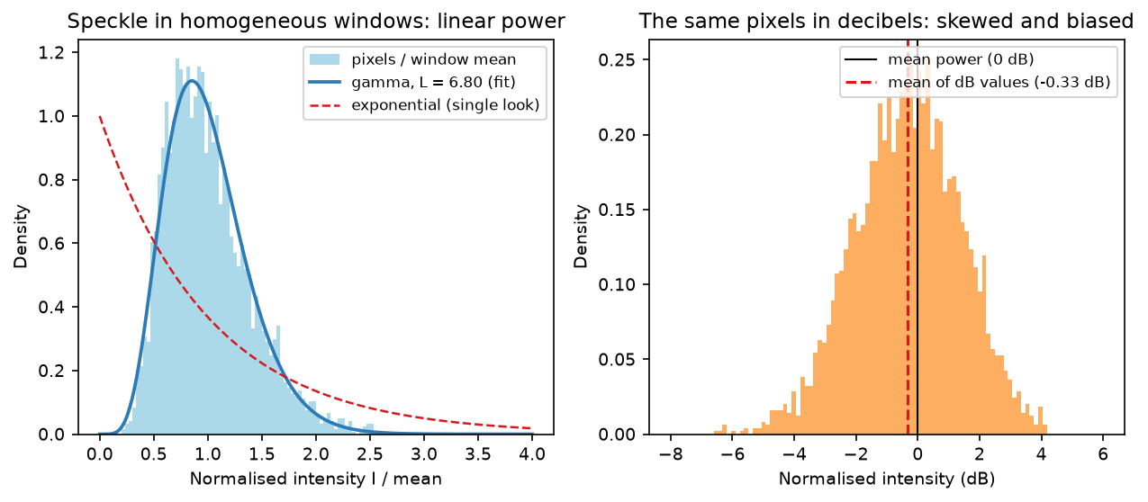
Why filter in linear power, not decibels

Decibels (10 · log10(I)) are handy for display because they compress a range of 0.002 to 100 into −27 to +20 dB. But the logarithm is non-linear, and the mean of the logs is not the log of the mean. For gamma-distributed speckle the bias has an exact formula:

E[10 log10 n] = (10 / ln 10) · (ψ(L) − ln L)

where ψ is the digamma function. For L = 6.8 that is −0.33 dB, exactly what we measured above. For single-look data (L = 1) it is −2.5 dB. Filtering in dB also breaks the speckle model: the filters below assume multiplicative noise with a known CV, whereas in dB the noise becomes additive with a different, skewed distribution. The script runs the same 7 × 7 boxcar both ways:

raw image         : mean over homogeneous windows -11.63 dB; whole-chip mean power  -8.86 dB
boxcar in linear  : mean over homogeneous windows -11.63 dB; whole-chip mean power  -8.86 dB
boxcar in dB      : mean over homogeneous windows -11.91 dB; whole-chip mean power  -9.58 dB

Filtering linear power preserves the mean backscatter exactly. Filtering dB values loses 0.3 dB in uniform areas and 0.7 dB over the whole scene, where bright point targets dominate the mean power. That is enough to shift a water threshold or a crop-growth curve.

Step 3: six speckle filters in NumPy and SciPy

Every filter below uses the same local statistics, the mean and variance in a moving window, which scipy.ndimage.uniform_filter computes in a few milliseconds:

def moments(x, size):
    mean = ndimage.uniform_filter(x, size)
    var = np.maximum(ndimage.uniform_filter(x * x, size) - mean * mean, 0)
    return mean, var


def boxcar(x, size=7, enl=None):
    return ndimage.uniform_filter(fill_nan(x), size)

fill_nan replaces no-data pixels with the image median so they do not spread; the script puts the NaNs back after filtering. The boxcar (moving average) is the baseline: it reduces speckle in proportion to the number of pixels averaged, and blurs everything else just as much.

Lee (1980)

The Lee filter estimates how much of the local variance is real signal and how much is speckle. In a uniform window, all the variance is speckle (var ≈ mean² / L), so k ≈ 0 and the output is the local mean. At an edge, the variance is much larger than speckle alone explains, so k → 1 and the pixel is left almost unchanged:

def lee(x, size=7, enl=4.4):
    """Lee (1980): out = mean + k (x - mean), k from the local variance in excess of pure speckle."""
    x = fill_nan(x)
    mean, var = moments(x, size)
    cu2 = 1 / enl                                   # speckle variance (coefficient of variation squared)
    var_x = np.maximum((var - mean ** 2 * cu2) / (1 + cu2), 0)
    k = var_x / np.maximum(var, 1e-12)
    return mean + k * (x - mean)

Enhanced Lee and Gamma-MAP (Lopes et al., 1990)

Both use two thresholds on the local CV, Ci. Below Cu = 1/√L the window is treated as pure speckle and replaced by its mean; above Cmax = √(1 + 2/L) it is treated as a point target and kept as it is. In between, enhanced Lee blends the two with an exponential weight. Gamma-MAP assumes the true backscatter itself follows a gamma distribution and computes the maximum a posteriori estimate, which is the root of a quadratic:

def enhanced_lee(x, size=7, enl=4.4, damping=1.0):
    """Enhanced Lee (Lopes et al. 1990): full smoothing below Cu, none above Cmax, exponential in between."""
    x = fill_nan(x)
    mean, var = moments(x, size)
    ci = np.sqrt(var) / np.maximum(mean, 1e-12)
    cu, cmax = 1 / np.sqrt(enl), np.sqrt(1 + 2 / enl)
    c = np.clip(ci, cu, cmax - 1e-6)
    w = np.exp(-damping * (c - cu) / (cmax - c))     # 1 in homogeneous areas, 0 at point targets
    out = mean * w + x * (1 - w)
    return np.where(ci >= cmax, x, out)


def gamma_map(x, size=7, enl=4.4):
    """Gamma-MAP (Lopes et al. 1990): maximum a posteriori estimate with a gamma-distributed scene."""
    x = fill_nan(x)
    mean, var = moments(x, size)
    ci2 = var / np.maximum(mean ** 2, 1e-12)
    cu2, cmax2 = 1 / enl, 1 + 2 / enl
    with np.errstate(divide="ignore", invalid="ignore"):
        alpha = (1 + cu2) / (ci2 - cu2)
        b = alpha - enl - 1
        out = (b * mean + np.sqrt(np.maximum(mean ** 2 * b ** 2 + 4 * alpha * enl * mean * x, 0))) / (2 * alpha)
    return np.where(ci2 <= cu2, mean, np.where(ci2 >= cmax2, x, out))

Frost (1982)

The Frost filter is a weighted mean whose weights decay exponentially with distance from the centre pixel. The decay rate is proportional to the local CV², so the kernel is wide and flat in uniform areas and shrinks to almost a single pixel at edges. Because the kernel changes at every pixel, it cannot use uniform_filter; we loop over the 49 offsets of the 7 × 7 window instead, which is still fully vectorised over the image:

def frost(x, size=7, enl=None, damping=2.0):
    """Frost (1982): exponentially weighted mean, with a decay that grows with local heterogeneity."""
    x = fill_nan(x)
    mean, var = moments(x, size)
    a = damping * var / np.maximum(mean ** 2, 1e-12)
    h = size // 2
    pad = np.pad(x, h, mode="reflect")
    num, den = np.zeros_like(x), np.zeros_like(x)
    for dy in range(-h, h + 1):
        for dx in range(-h, h + 1):
            w = np.exp(-a * np.hypot(dy, dx))
            num += w * pad[h + dy:h + dy + x.shape[0], h + dx:h + dx + x.shape[1]]
            den += w
    return num / den

Refined Lee (Lee, 1981)

The plain Lee filter uses a square window, so near an edge the window straddles both sides and the filter simply smooths less. Refined Lee first finds the edge direction, then computes the Lee statistics only from the half of a 7 × 7 window that lies on the same side of the edge as the centre pixel. It splits the window into a 3 × 3 grid of 3 × 3 blocks, takes the strongest of four gradients (vertical, horizontal and two diagonals) between their means, and chooses one of eight directional half-windows:

def refined_lee(x, enl=4.4, size=7):
    """Refined Lee (Lee 1981): Lee statistics from the edge-aligned half of a 7 x 7 window."""
    x = fill_nan(x)
    m3 = ndimage.uniform_filter(x, 3)
    pad = np.pad(m3, 2, mode="reflect")
    s = [[pad[2 + 2 * (r - 1):2 + 2 * (r - 1) + x.shape[0], 2 + 2 * (c - 1):2 + 2 * (c - 1) + x.shape[1]]
          for c in range(3)] for r in range(3)]                           # 3 x 3 grid of 3 x 3 sub-window means
    grads = np.stack([abs(s[0][1] - s[2][1]), abs(s[1][0] - s[1][2]),   # vertical, horizontal
                      abs(s[0][0] - s[2][2]), abs(s[0][2] - s[2][0])])  # two diagonals
    pairs = [("N", "S", s[0][1], s[2][1]), ("W", "E", s[1][0], s[1][2]),
             ("NW", "SE", s[0][0], s[2][2]), ("NE", "SW", s[0][2], s[2][0])]
    best = np.argmax(grads, axis=0)
    masks = _refined_masks()                     # eight 7 x 7 boolean half-windows, e.g. "N": rows 0-3
    mean, var = np.empty_like(x), np.empty_like(x)
    for d, (a, b, sa, sb) in enumerate(pairs):
        side_a = abs(s[1][1] - sa) <= abs(s[1][1] - sb)                 # the centre belongs to the closer side
        for name, sel in ((a, side_a), (b, ~side_a)):
            k = masks[name].astype("float32") / masks[name].sum()
            mu = ndimage.correlate(x, k, mode="reflect")
            v = np.maximum(ndimage.correlate(x * x, k, mode="reflect") - mu * mu, 0)
            pick = (best == d) & sel
            mean[pick], var[pick] = mu[pick], v[pick]
    cu2 = 1 / enl
    var_x = np.maximum((var - mean ** 2 * cu2) / (1 + cu2), 0)
    return mean + var_x / np.maximum(var, 1e-12) * (x - mean)

Rather than looping over pixels, it computes all eight directional means with ndimage.correlate over the whole image and then picks, per pixel, the one that applies. That is wasteful (eight convolutions where one would do per pixel) but needs no compiled code.

We time each filter on the full 1156 × 1316 chip (best of three runs):

filtering with a 7 x 7 window and ENL = 6.7
Boxcar 7×7         15 ms  ( 98.9 Mpixel/s)
Lee                37 ms  ( 41.5 Mpixel/s)
Refined Lee       464 ms  (  3.3 Mpixel/s)
Enhanced Lee       58 ms  ( 26.0 Mpixel/s)
Frost             679 ms  (  2.2 Mpixel/s)
Gamma-MAP          52 ms  ( 29.3 Mpixel/s)

At 30 to 40 megapixels per second, Lee and Gamma-MAP would filter a whole 25,000 × 17,000 pixel Sentinel-1 RTC scene in about 15 seconds on one core, if it fits in memory. Refined Lee and Frost are 10 to 15 times slower in this NumPy form; Numba or a compiled implementation would close most of the gap.

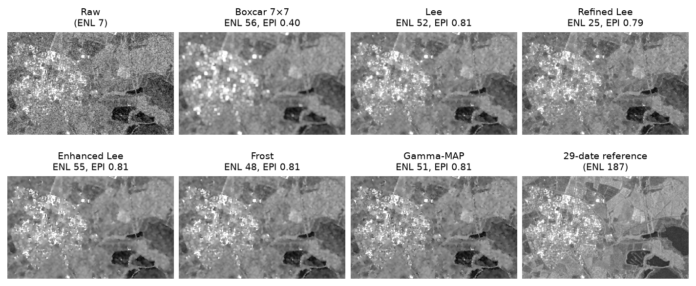
Step 4: score the filters

A good speckle filter does two things that pull against each other: it smooths uniform areas and it keeps edges and point targets. We measure both, plus a check that nothing else was removed:

• ENL in the eight homogeneous windows: higher means more speckle removed.
• Edge-preservation index (EPI), after Sattar et al. (1997): the correlation between the high-pass detail of the filtered image and of the speckle-free reference, on the 10% of pixels with the strongest edges in the reference. 1 is perfect; a filter that blurs edges, or adds false ones, scores lower.
• The ratio image, raw ÷ filtered. If a filter removed only speckle, the ratio is pure speckle: mean 1, standard deviation 1/√L (0.386 here), and no visible structure.

gy, gx = ndimage.sobel(ref_db, 0), ndimage.sobel(ref_db, 1)
edges = np.hypot(gx, gy) > np.nanpercentile(np.hypot(gx, gy), 90)     # strongest 10% of reference edges


def highpass(x_db):
    x_db = np.nan_to_num(x_db)
    return x_db - ndimage.gaussian_filter(x_db, 3)


def epi(x):
    a, b = highpass(db(x))[edges], highpass(ref_db)[edges]
    a, b = a - a.mean(), b - b.mean()
    return float((a * b).sum() / np.sqrt((a * a).sum() * (b * b).sum()))

edge pixels (top 10% Sobel gradient of the reference): 152,130
               ENL  ENL water  ENL land    EPI  ratio mean  ratio std  RMSE vs ref (dB)     ms
filter
None (raw)     6.7        6.2       7.2  0.781       1.000      0.000              2.14    0.0
Boxcar 7×7    56.4       40.7      72.1  0.401       0.977      0.402              1.58   15.0
Lee           52.1       35.7      68.4  0.811       0.970      0.299              1.49   37.0
Refined Lee   24.7       19.3      30.1  0.790       1.022      0.287              1.71  464.0
Enhanced Lee  55.4       39.3      71.4  0.806       0.978      0.324              1.49   58.0
Frost         48.0       34.5      61.6  0.808       0.974      0.315              1.48  679.0
Gamma-MAP     50.6       34.7      66.4  0.809       1.011      0.294              1.63   52.0
(pure speckle would give a ratio image with mean 1 and std 0.386)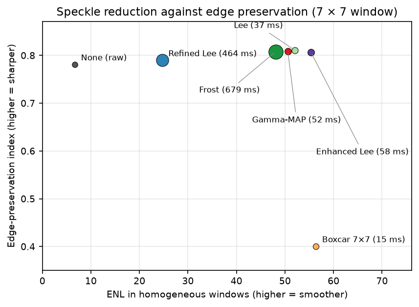

What the numbers say:

• The boxcar removes the most speckle (ENL 56) but halves the edge-preservation index (0.78 to 0.40). Its ratio-image standard deviation of 0.402 is higher than pure speckle (0.386): it has removed real structure as well.
• Lee, enhanced Lee, Frost and Gamma-MAP are almost indistinguishable on these metrics: ENL 48 to 55, nearly as smooth as the boxcar, with an EPI of 0.81, slightly better than the raw image because the speckle on either side of each edge has gone. Lee and Gamma-MAP are the cheapest.
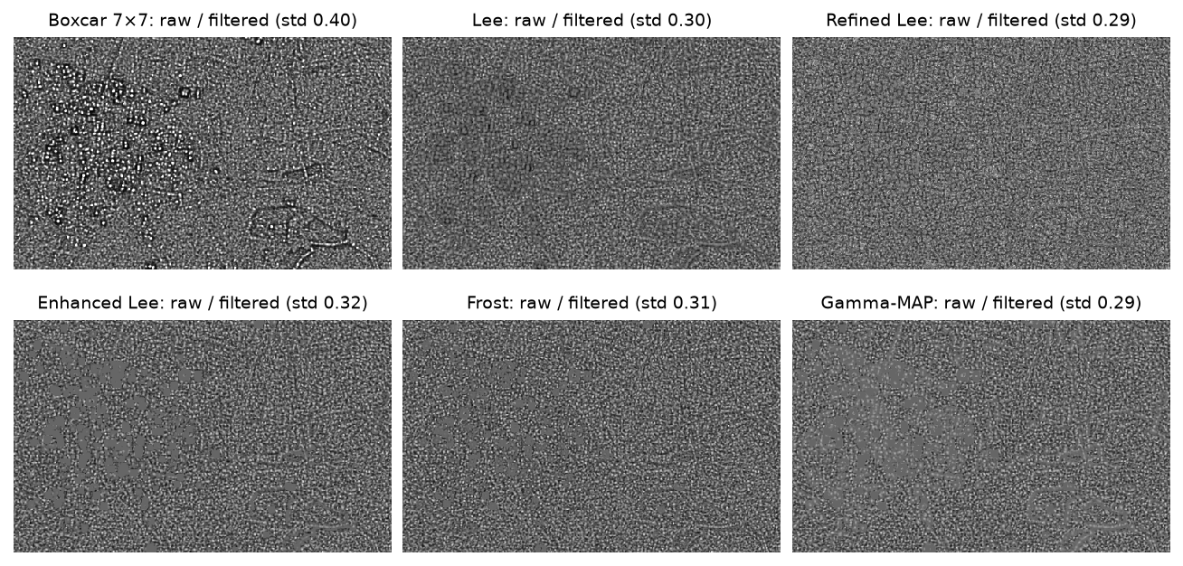
• Refined Lee smooths uniform areas less (ENL 25), because each directional half-window holds only 28 pixels and the variance estimate is noisier. In return, it gives the cleanest, straightest boundaries in the comparison figure. A larger window, or a second pass, raises its ENL.
• All the adaptive filters leave some speckle (ratio std 0.29 to 0.32, below 0.386). That is by design: in windows that look heterogeneous, they keep part of the original pixel.
• No filter comes close to the multi-temporal reference (ENL 187). If you have a stack of dates and the landscape is stable, averaging dates beats any single-image filter. Use spatial filters when you need one date, such as for a flood or a ship.

Step 5: look at the edges

Numbers hide what happens at individual edges. A transect from west to east across a lagoon, a strip of land and the open reservoir shows it directly:

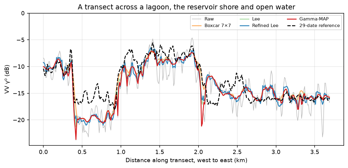
The ratio images show the same thing for the whole zoom area. The boxcar’s ratio image shows the outlines of buildings, roads and lagoon shores: the structure it smoothed away. The adaptive filters’ ratio images look like pure noise, with only faint traces of the strongest edges, and flat grey patches where enhanced Lee and Gamma-MAP decided that a pixel was a point target and left it alone.

Limitations

• One scene, one window size. We tested a 7 × 7 window on one winter scene with a lot of water. A 5 × 5 window keeps more detail; 9 × 9 or 11 × 11 smooths more. Repeat the scoring on your own area before choosing.
• The reference is not perfect truth. The 29-date mean blends six months of change: wet and dry soil, crops emerging, calm and windy water. That is why the “RMSE vs ref” column flatters no filter, and why EPI is measured only on the strongest edges, which are mostly permanent.
• ENL is a parameter, not a constant. It varies with the product, the processor and the polarisation. VH has lower backscatter and gets closer to the noise floor, where the speckle model breaks down.
• These filters assume fully developed speckle. In towns, a few strong scatterers dominate each pixel and the statistics are not gamma. That is why cities stay noisy after filtering, and why many ship detectors model sea clutter with K or G⁰ distributions instead.
• Modern alternatives. Non-local means, BM3D-based SAR-BM3D, and deep learning despecklers (for example SAR2SAR or MERLIN, trained without clean targets) beat all the classic filters on both ENL and edges, at the cost of more computation and dependencies.

Frequently asked questions

What is the best speckle filter for Sentinel-1?

For most work, a 7 × 7 Lee or Gamma-MAP filter: in this test both reached an ENL above 50 with an edge-preservation index of 0.81, in under 60 ms per 1.5 megapixels. Use refined Lee when sharp, straight boundaries matter more than smooth fields, for example for field or shoreline mapping. If you have a time series and the landscape is stable, averaging dates (multi-temporal filtering) beats any single-image filter.

How do I apply a Lee filter to Sentinel-1 in Python?

Compute the local mean and variance with scipy.ndimage.uniform_filter on the linear VV or VH values, then apply out = mean + k * (img - mean) with k = var_x / var and var_x = (var - mean**2 / ENL) / (1 + 1/ENL), as in the function above. Measure the ENL from a uniform area of your own image. Convert to dB afterwards.

Should I apply speckle filters to dB or linear values?

Linear. Speckle is multiplicative and gamma-distributed in linear power, which is what the filters assume. Averaging dB values gives a biased result: −0.33 dB for this 6.7-look data, −2.5 dB for single-look data. Here a boxcar in dB lowered the scene mean by 0.7 dB.

What does ENL mean in SAR?

The equivalent number of looks: mean² ÷ variance of intensity over an area of uniform backscatter. It tells you how many independent looks would produce the speckle you see. Raw Sentinel-1 RTC measured 6.7 here; a 7 × 7 Lee filter raised it to 52; averaging 29 dates gave 187. Higher means smoother.

Does Google Earth Engine or SNAP have speckle filters?

Yes. ESA SNAP offers Lee, refined Lee, Lee Sigma, Frost, Gamma-MAP and others in its Speckle Filter operator, and Earth Engine has focal_mean and community implementations of refined Lee and Gamma-MAP. Writing them in NumPy, as here, lets you run them anywhere, check what they do, and score them on your own data.

Next steps

• Put the filters to work: thresholding a filtered image is the core of Sentinel-1 SAR flood mapping in Python.
• Detect ships, which speckle filters would blur away, with an adaptive threshold in Sentinel-1 ship detection in Python with CFAR.
• Use multi-temporal filtering and field averages to follow crops through the season in Sentinel-1 crop monitoring in Python.
• Go from amplitude to phase, where speckle becomes decorrelation, in InSAR ground subsidence in Python.
• Feed filtered backscatter into a classifier with Land cover classification with random forest.
• Test whether seasonal Sentinel-1 backscatter improves a habitat classifier in LightGBM habitat classification with Sentinel-1, Sentinel-2 and terrain, Part 2 of our AI habitat classification series.

Data and licences

• Sentinel-1 RTC: contains modified Copernicus Sentinel data 2025–2026, processed by ESA; radiometric terrain correction by Catalyst/Microsoft. Licensed CC BY 4.0. Accessed from the Microsoft Planetary Computer on 21 October 2026.
• References: Lee, J.-S. (1980), IEEE Transactions on Pattern Analysis and Machine Intelligence 2(2); Lee, J.-S. (1981), “Refined filtering of image noise using local statistics”, Computer Graphics and Image Processing 15(4); Frost, V. S. et al. (1982), IEEE Transactions on Pattern Analysis and Machine Intelligence 4(2); Lopes, A., Touzi, R. and Nezry, E. (1990), “Adaptive speckle filters and scene heterogeneity”, IEEE Transactions on Geoscience and Remote Sensing 28(6); Sattar, F. et al. (1997), IEEE Transactions on Image Processing 6(6).
• Code: speckle_filters.py, tested with Python 3.12.0, pystac-client 0.9.1, planetary-computer 1.0.0, rasterio 1.5.2, NumPy 2.5.4 and SciPy 1.18.1.