Deforestation detection in Python with Global Forest Change data (Rondônia, 2001–2025)
Map forest loss and deforestation in Python with the Hansen/UMD Global Forest Change v1.13 data: read the open tiles with no login, compute loss by year in hectares with correct pixel areas, compare Landsat and Sentinel-2 images before and after, and check the GFC loss year against Sentinel-2 NBR and MODIS burned area for central Rondônia, Brazil.
- Level
- Intermediate
- Tested with
- Python 3.12
- Source code
- Download scripts
Key takeaways
- Hansen/UMD Global Forest Change v1.13 maps tree cover in 2000 and the year of loss for 2001–2025 at 0.00025° (about 30 m). It is free, needs no login and can be read straight from Google Cloud Storage with rasterio.
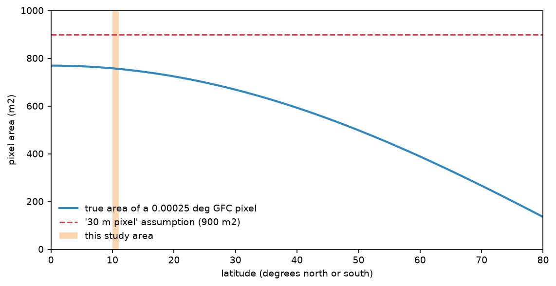
- GFC pixels are not equal area. At 10.5°S a pixel covers 757 m², not 900 m², so multiplying pixel counts by 0.09 ha overstates every area here by 18.9%. Compute each row's area on the ellipsoid instead.
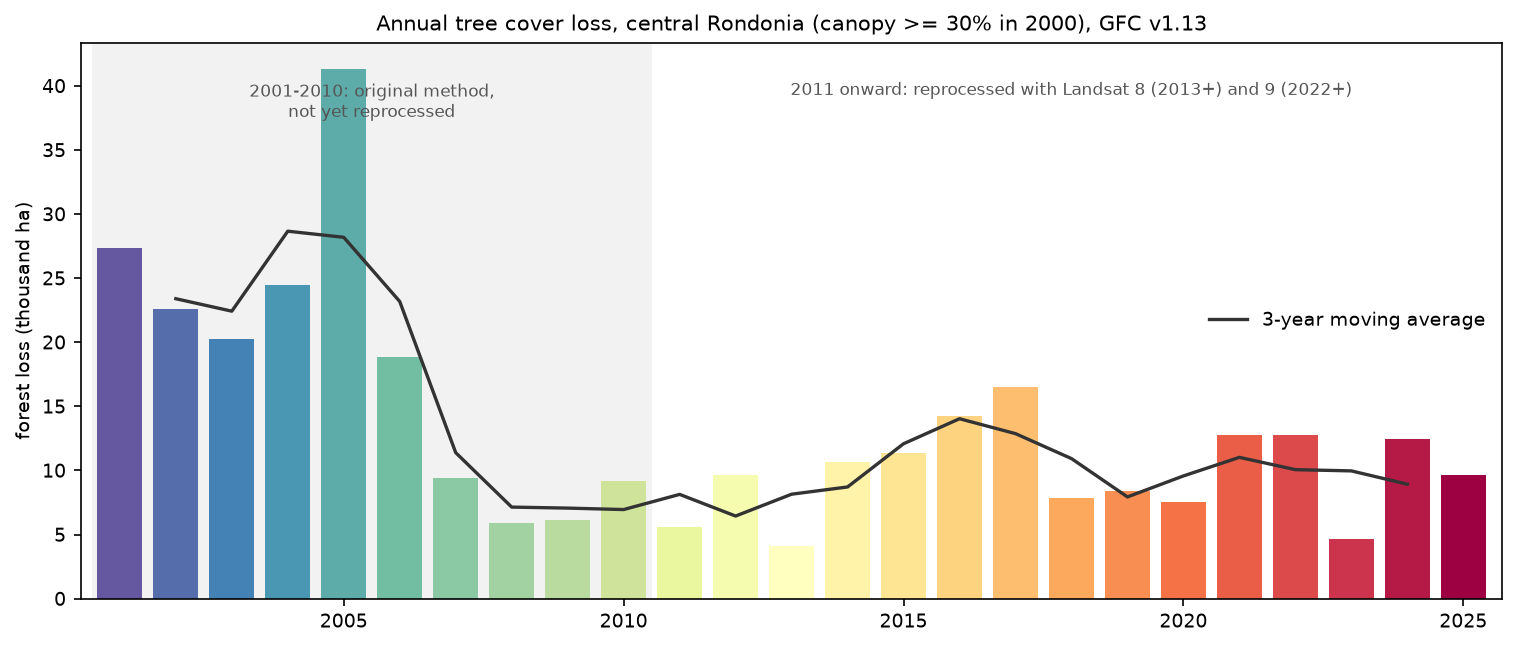
- In a 1° × 1° block of central Rondônia, 333,606 ha of the 1,007,753 ha of forest in 2000 (33.1%) was lost by 2025. Loss peaked at 41,281 ha in 2005, fell to about 9,600 ha a year in 2011–2020 and averaged 10,460 ha a year in 2021–2025.
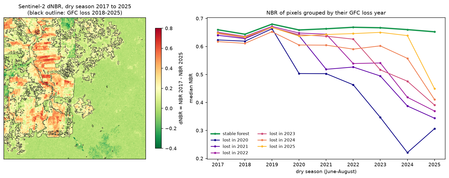
- Sentinel-2 dry-season NBR confirms the loss: the median NBR of stable forest stays at 0.64–0.68, while pixels lost in 2020 fall from 0.66 to 0.22 by 2024. The biggest annual NBR drop lands in the GFC year or the year after for 51.5% of loss pixels.
- GFC 'loss' is any removal of tree canopy, not only permanent deforestation. It includes fire, plantation harvest and natural disturbance. The method changed in 2011, and the loss pixel counts are not unbiased area estimates.
Before you start
- Comfortable with NumPy arrays and rasterio (the Sentinel-2 Lake Mead tutorial introduces STAC searches and Cloud Optimised GeoTIFFs)
- Python 3.10+ with rasterio, numpy, pandas, pyproj, shapely, pystac-client, planetary-computer and matplotlib
- An internet connection: the forest data comes from a public Google Cloud Storage bucket and the imagery from the Microsoft Planetary Computer, and neither needs an account
Short answer: to detect deforestation in Python, start from the Hansen/UMD Global Forest Change (GFC) data rather than training your own classifier. Read the treecover2000, lossyear and datamask layers for your area from the public bucket at storage.googleapis.com/earthenginepartners-hansen/GFC-2025-v1.13/ with rasterio. Define forest as land with at least 30% canopy in 2000, and count each loss year (1–25 = 2001–2025) inside that mask. Multiply by the true area of each pixel, which you calculate row by row on the WGS84 ellipsoid, not by 0.09 ha. Then check the result against imagery. For a 1° × 1° block of central Rondônia, Brazil, this gives 333,606 ha of forest loss from 2001 to 2025, a third of the forest that stood in 2000.
Rondônia, in the south-western Brazilian Amazon, is one of the most studied deforestation frontiers in the world. Since the BR-364 highway was paved in the 1980s, settlement projects have cut the forest into the “fishbone” pattern that you can see from space: roads every few kilometres, with farms cleared back from each road. We study the block from 10°S to 11°S and 64°W to 63°W, around the towns of Buritis and Campo Novo de Rondônia. Its northern half is the settlement frontier. The unbroken forest to the south lies mostly in protected areas, including the Uru-Eu-Wau-Wau Indigenous Territory.
You will learn how to:
- read windows of the GFC v1.13 GeoTIFFs straight from Google Cloud Storage, with no login;
- compute true pixel areas and see why multiplying by 0.09 ha is wrong;
- tabulate forest loss by year in hectares, with a 3-year moving average and canopy thresholds;
- make a before-and-after comparison with Landsat 7 (2000) and Sentinel-2 (2017 and 2025) from the Planetary Computer;
- check the GFC loss year against a Sentinel-2 NBR time series;
- estimate how much of the loss burned, using MODIS burned area.
All outputs below are real results from deforestation_gfc.py, run on 19 October 2026 with Python 3.12, rasterio 1.5.2, numpy 2.5.4, pyproj 3.8.0, pystac-client 0.9.0 and planetary-computer 1.0.0.
What the Global Forest Change data is
Hansen and colleagues at the University of Maryland published the first global, 30 m map of forest change in Science in 2013. They classified every Landsat image from 2000 to 2012 in Google Earth Engine. The data has been extended every year since. Version 1.13 covers 2001–2025 and is the latest version on the public bucket.
Each 10° × 10° tile has several layers:
| Layer | Meaning |
|---|---|
treecover2000 |
Canopy closure for all vegetation taller than 5 m in 2000, 0–100% |
lossyear |
Year of stand-replacing loss: 0 = none, 1–25 = 2001–2025 |
gain |
Tree cover gain during 2000–2012 only (1 = gain) |
datamask |
0 = no data, 1 = land, 2 = permanent water |
first, last |
Cloud-free Landsat composites for about 2000 and the latest year |
Tiles are named after their north-west corner. Our block, 10–11°S and 63–64°W, is inside the tile that runs from 10°S to 20°S and 70°W to 60°W, so it is 10S_070W.
Step 1: read the GFC layers for the study area
The tiles are 40,000 × 40,000 pixels. You don’t need to download them whole: GDAL’s /vsicurl/ handler reads only the bytes that a window needs. We read a 1° window once and cache it locally as a tiled GeoTIFF:
VERSION = "GFC-2025-v1.13"GFC = f"https://storage.googleapis.com/earthenginepartners-hansen/{VERSION}/Hansen_{VERSION}_{{layer}}_10S_070W.tif"AOI = (-64.0, -11.0, -63.0, -10.0)   # lon/lat: central Rondonia around Buritis and Campo Novo de RondoniaRES = 0.00025                        # GFC pixel size in degrees (0.9 arc-seconds)FOREST_CANOPY = 30                   # % canopy cover in 2000 that counts as forest (the GFW default)

def read_gfc(layer):    """Window of one 10x10 degree GFC tile, cached locally as a tiled GeoTIFF."""    path = DATA / f"{VERSION}_{layer}_rondonia.tif"    if not path.exists():        with rasterio.open("/vsicurl/" + GFC.format(layer=layer)) as src:            win = from_bounds(*AOI, transform=src.transform)            arr = src.read(1, window=win)            prof = src.profile | {"width": arr.shape[1], "height": arr.shape[0], "transform": src.window_transform(win),                                  "tiled": True, "blockxsize": 512, "blockysize": 512, "compress": "deflate"}        with rasterio.open(path, "w", **prof) as dst:            dst.write(arr, 1)    with rasterio.open(path) as src:        return src.read(1), src.transform

treecover, transform = read_gfc("treecover2000")lossyear, _ = read_gfc("lossyear")lossyear = lossyear.astype(np.int16) # uint8 overflows when we add 2000datamask, _ = read_gfc("datamask")GFC-2025-v1.13: 4000 x 4000 pixels of 0.00025 deg over lon -64.0..-63.0, lat -11.0..-10.0lossyear values: 0..25 (0 = no loss, 1..25 = 2001..2025)datamask: land 99.99%, water 0.01%, no data 0.00%Step 2: compute the true area of each pixel
A GFC pixel is 0.00025° on each side, which is often described as “30 m”. That is only roughly true at the equator. The north–south size stays almost constant, but the east–west width shrinks with the cosine of latitude. We calculate the exact area of one pixel in every row with pyproj.Geod, which works on the WGS84 ellipsoid:
geod = Geod(ellps="WGS84")lats = transform.f + transform.e * np.arange(H + 1)            # row edges, north to southrow_area = np.array([abs(geod.polygon_area_perimeter([0, RES, RES, 0], [lats[i], lats[i], lats[i + 1], lats[i + 1]])[0])                     for i in range(H)])                         # m2 of one pixel in each rowarea_ha = np.repeat(row_area[:, None] / 1e4, W, axis=1).astype(np.float32)   # hectares per pixel

def ha(mask):    return float(area_ha[mask].sum())

land = datamask == 1forest2000 = land & (treecover >= FOREST_CANOPY)at 10.5 S one pixel is 27.37 m wide x 27.65 m tall = 756.8 m2 (0.0757 ha)row areas range 755.6..757.9 m2 across the AOI pixel area at 0.0 deg: 769.3 m2 (0.85 x a 30 m square) pixel area at 10.5 deg: 756.8 m2 (0.84 x a 30 m square) pixel area at 30.0 deg: 668.5 m2 (0.74 x a 30 m square) pixel area at 50.0 deg: 498.4 m2 (0.55 x a 30 m square) pixel area at 60.0 deg: 388.5 m2 (0.43 x a 30 m square) pixel area at 70.0 deg: 266.3 m2 (0.30 x a 30 m square)AOI land area 1,210,727 ha; forest (>= 30% canopy) in 2000 1,007,753 ha (83.2% of land)pixel count x 0.09 ha would give 1,198,664 ha, +18.9% too muchEven at the equator, a 0.00025° pixel is only 27.8 m across, so the “30 m pixel” shortcut overstates area by 17% everywhere. The error grows with latitude: in a boreal forest at 60°N it more than doubles the true figure.
Step 3: forest loss by year in hectares
With an area for every pixel, the loss for each year is a weighted histogram of lossyear inside the 2000 forest mask. np.bincount does it in one call:
years = np.arange(2001, 2026)loss = forest2000 & (lossyear > 0)by_year = np.bincount(lossyear[forest2000].ravel(), weights=area_ha[forest2000].ravel(), minlength=26)[1:26]table = pd.DataFrame({"year": years, "loss_ha": by_year})table["pct_of_2000_forest"] = 100 * table.loss_ha / ha(forest2000)table["moving_avg_3yr"] = table.loss_ha.rolling(3, center=True).mean() year loss_ha pct_of_2000_forest moving_avg_3yr 2001 27,360.5 2.7 NaN 2002 22,565.0 2.2 23,398.2 2003 20,269.1 2.0 22,426.4 2004 24,445.3 2.4 28,665.0 2005 41,280.8 4.1 28,187.9 2006 18,837.7 1.9 23,180.7 2007 9,423.7 0.9 11,388.7 2008 5,904.6 0.6 7,142.8 2009 6,100.2 0.6 7,063.9 2010 9,187.1 0.9 6,951.3 2011 5,566.7 0.6 8,134.4 2012 9,649.4 1.0 6,445.2 2013 4,119.6 0.4 8,148.4 2014 10,676.3 1.1 8,713.9 2015 11,345.8 1.1 12,084.4 2016 14,231.0 1.4 14,036.1 2017 16,531.4 1.6 12,873.1 2018 7,856.9 0.8 10,926.6 2019 8,391.5 0.8 7,936.8 2020 7,562.0 0.8 9,573.5 2021 12,767.1 1.3 11,023.6 2022 12,741.8 1.3 10,063.4 2023 4,681.3 0.5 9,967.1 2024 12,478.2 1.2 8,931.0 2025 9,633.4 1.0 NaNtotal 2001-2025: 333,606 ha = 33.1% of the 2000 forest; peak 2005 (41,281 ha)2001-2010 mean 18,537 ha/yr; 2011-2020 mean 9,593 ha/yr; 2021-2025 mean 10,460 ha/yrcanopy threshold 10%: forest 2000 1,023,246 ha, loss 2001-2025 335,496 hacanopy threshold 30%: forest 2000 1,007,753 ha, loss 2001-2025 333,606 hacanopy threshold 50%: forest 2000 987,944 ha, loss 2001-2025 329,503 hacanopy threshold 75%: forest 2000 942,816 ha, loss 2001-2025 313,231 haloss pixels outside the 30% forest mask: 7,487 haA third of the forest that stood in this block in 2000 had gone by 2025. The timeline matches what is known about the Brazilian Amazon as a whole: a peak in the early 2000s (Brazil’s own PRODES system recorded its post-1995 maximum in 2004), a sharp fall after the 2004 action plan against deforestation and the 2008 credit restrictions, then a rise again from the mid-2010s.
In dense tropical forest the canopy threshold matters little: going from 10% to 50% changes the total loss by less than 2%. In savanna, dry forest or farmland with scattered trees it can change the answer several times over, so always state the threshold you used.
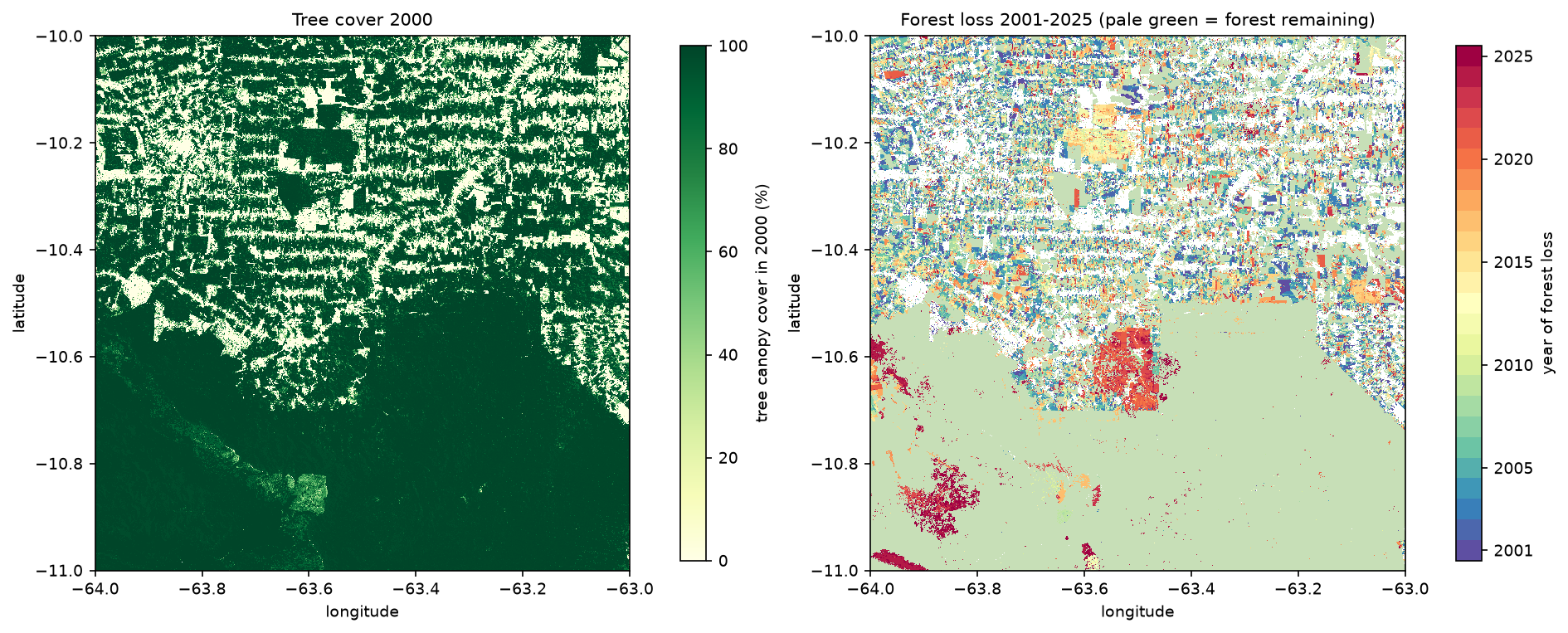
Look at the shapes as well as the colours. Clearing for pasture makes straight-edged blocks along the roads, like the large orange-red rectangle in the centre of the map. The irregular dark-red patches inside the southern forest, lost in 2024 and 2025, have the ragged outline of fire scars instead.
Step 4: before and after imagery from the Planetary Computer
Numbers are more convincing when you can see them. We pick the 480 × 480-pixel (about 13 × 13 km) window with the most loss between 2018 and 2024. It is about 15 km east of Campo Novo de Rondônia:
zoom: lon -63.520..-63.400, lat -10.720..-10.600 (480 x 480 GFC pixels)forest 2000 17,172 ha; loss 2001-2017 877 ha; loss 2018-2024 4,807 ha; loss 2025 884 haSentinel-2 only starts in 2015, so for the “before” image we use Landsat 7 from the dry season of 2000, the year that treecover2000 describes. Both are on the Microsoft Planetary Computer, which needs no account. The planetary_computer.sign_inplace modifier adds the short-lived access tokens. WarpedVRT reprojects each band from UTM straight onto the GFC lat/lon grid, so the imagery and the loss map line up pixel for pixel:
catalog = pystac_client.Client.open(STAC_URL, modifier=planetary_computer.sign_inplace)

def read_to_grid(href, bounds, shape, resampling=Resampling.average, dtype="float32"):    """Read a COG band straight onto our lat/lon grid (GFC pixels) with GDAL's warper."""    t = from_origin(bounds[0], bounds[3], RES, RES)    with rasterio.open(href) as src, WarpedVRT(src, crs="EPSG:4326", transform=t, width=shape[1], height=shape[0],                                              resampling=resampling) as vrt:        return vrt.read(1).astype(dtype)

def s2_reflectance(item, band, bounds, shape):    dn = read_to_grid(item.assets[band].href, bounds, shape)    offset = 1000 if item.properties.get("s2:processing_baseline", "00.00") >= "04.00" else 0    return np.where(dn == 0, np.nan, (dn - offset) / 10000)

def best_s2(year, bounds, months="06-01/08-31", n=3):    items = catalog.search(collections=["sentinel-2-l2a"], bbox=bounds, datetime=f"{year}-{months.replace('/', f'/{year}-')}",                           query={"eo:cloud_cover": {"lt": 20}}).item_collection()    items = sorted((it for it in items if shape(it.geometry).contains(box(*bounds))),                   key=lambda it: it.properties["eo:cloud_cover"])    return items[:n]

landsat = catalog.search(collections=["landsat-c2-l2"], bbox=zb, datetime="2000-06-01/2000-08-31", query={"platform": {"eq": "landsat-7"}, "eo:cloud_cover": {"lt": 5}}).item_collection()ls = sorted(landsat, key=lambda it: (it.properties["eo:cloud_cover"], it.datetime))[0]ls_rgb = np.dstack([read_to_grid(ls.assets[b].href, zb, (Z, Z)) * 0.0000275 - 0.2 for b in ("red", "green", "blue")])s2_before, s2_after = best_s2(2017, zb, n=1)[0], best_s2(2025, zb, n=1)[0]Landsat 7 before: LE07_L2SP_232067_20000612_02_T1 cloud 0.0%Sentinel-2 before: S2B_MSIL2A_20170720T142749_R053_T20LMP_20210210T120110 cloud 0.0% baseline 02.12Sentinel-2 after: S2C_MSIL2A_20250703T142811_R053_T20LMP_20250703T194403 cloud 0.0% baseline 05.11June to August is the dry season in Rondônia, so clear images are easy to find. We keep only scenes whose footprint contains the whole window. That avoids the no-data edges of a tile.
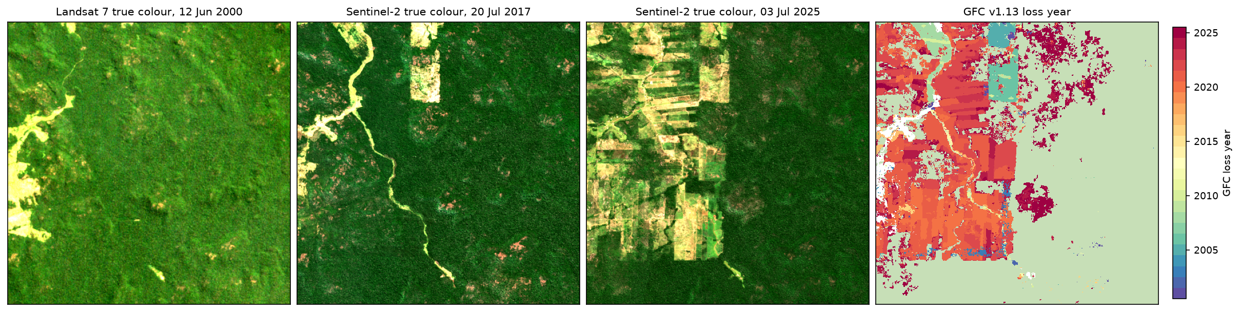
The match is good: the straight-edged blocks that appear between 2017 and 2025 are the orange and red pixels of the loss map. But look at the dark-red patches on the right of the loss map, recorded as loss in 2024 and 2025. In the July 2025 image that area still looks like forest, only slightly mottled. That is what canopy killed by fire looks like: the dead trees still stand, but GFC counts the canopy as lost.
Step 5: check the loss year with a Sentinel-2 NBR time series
GFC is a model output, so it is worth an independent check. The Normalised Burn Ratio, NBR = (B8A − B12) / (B8A + B12), is high over closed forest and drops when the canopy is opened or burned. We build a dry-season median NBR for each year from 2017 to 2025, using the three clearest Sentinel-2 scenes and masking cloud, shadow and cirrus with the SCL band. Then we follow pixels grouped by their GFC loss year:
def nbr_composite(items, bounds, shape):    """Median NBR of the clearest scenes, with cloud, shadow, cirrus and nodata masked by SCL."""    stack = []    for it in items:        scl = read_to_grid(it.assets["SCL"].href, bounds, shape, Resampling.nearest)        nir, swir = s2_reflectance(it, "B8A", bounds, shape), s2_reflectance(it, "B12", bounds, shape)        nbr = (nir - swir) / (nir + swir)        nbr[np.isin(scl, [0, 1, 3, 8, 9, 10])] = np.nan        stack.append(nbr)    return np.nanmedian(np.stack(stack), axis=0)

nbr_years = {}for yr in range(2017, 2026):    items = best_s2(yr, zb)    nbr_years[yr] = nbr_composite(items, zb, (Z, Z))stable = zf & (zly == 0)traj = {"stable forest": [np.nanmedian(nbr_years[y][stable]) for y in nbr_years]}for ly in range(18, 26):    m = zf & (zly == ly)    if m.sum() > 200:        traj[f"lost in {2000 + ly}"] = [np.nanmedian(nbr_years[y][m]) for y in nbr_years]
# year of the largest year-on-year NBR drop vs the GFC year, pixel by pixelyrs = np.array(list(nbr_years))cube = np.stack([nbr_years[y] for y in yrs])drops = cube[:-1] - cube[1:] # positive = NBR fell from year t to t+1valid = np.isfinite(drops).all(axis=0)drop_year = yrs[1:][np.nanargmax(np.where(np.isfinite(drops), drops, -9), axis=0)]sel = zf & (zly >= 18) & validdiff = drop_year[sel] - (zly[sel] + 2000)median NBR by year (rows: GFC class, columns: 2017..2025) stable forest 0.66 0.64 0.68 0.66 0.66 0.67 0.67 0.66 0.65 lost in 2020 0.62 0.62 0.66 0.50 0.50 0.46 0.35 0.22 0.31 lost in 2021 0.64 0.63 0.67 0.64 0.52 0.53 0.49 0.39 0.34 lost in 2022 0.65 0.64 0.67 0.65 0.64 0.54 0.54 0.42 0.37 lost in 2023 0.65 0.63 0.67 0.64 0.64 0.63 0.52 0.48 0.39 lost in 2024 0.62 0.61 0.65 0.61 0.60 0.59 0.60 0.56 0.41 lost in 2025 0.65 0.63 0.67 0.64 0.64 0.65 0.65 0.64 0.45loss pixels 2018-2025 with a full NBR record: 75,238largest annual NBR drop in the GFC year: 35.6%; one year later: 15.9%; one year earlier: 2.9%; further off: 45.6%largest drop >= 0.2 for 55.6% of GFC loss pixels vs 3.1% of stable-forest pixelsdNBR 2017->2025 median: stable forest 0.005, lost 2018-2025 0.225, lost 2001-2017 0.109Each group of loss pixels holds the stable-forest NBR of about 0.65 until its GFC year and then drops, so the loss years are right as a group. Pixel by pixel the timing is looser. The largest drop falls in the GFC year for 35.6% of pixels and in the following year for another 15.9%. There are two reasons for the lag:
- Our composites only cover June to August, but clearing and burning in Rondônia continue into September and October. Loss after August first shows up in next year’s composite.
- Clearing is often gradual: understorey first, then the big trees, then burning and pasture. The NBR of the 2020 group keeps falling until 2024. So the biggest single drop can come a year or two after GFC first records the loss.
Only 3.1% of stable-forest pixels have a drop of 0.2 or more, against 55.6% of loss pixels, so the NBR check also supports GFC’s “no loss” class.
Step 6: how much of the loss burned?
GFC loss in the Amazon is a mix of clear-cutting, fire and the two together, because cut forest is usually burned to make pasture. MODIS MCD64A1 maps burned area every month at 500 m, and it is also on the Planetary Computer. We reproject each monthly Burn_Date layer onto our grid and ask what share of each year’s GFC loss lies inside a burn scar from the same year:
for yr in range(2019, 2026): burned = np.zeros((H, W), dtype=bool) items = catalog.search(collections=["modis-64A1-061"], bbox=AOI, datetime=f"{yr}-01-01/{yr}-12-31").item_collection() for it in items: bd = read_to_grid(it.assets["Burn_Date"].href, (AOI[0], AOI[1], AOI[2], AOI[3]), (H, W), Resampling.nearest, dtype="int16") burned |= bd > 0 months = len({it.properties["start_datetime"][:7] for it in items}) m = forest2000 & (lossyear == yr - 2000) burn_rows.append((yr, months, ha(m), ha(m & burned), ha(burned & land))) year modis_months gfc_loss_ha loss_in_modis_burn_ha modis_burned_ha share_burned 2019 12 8,392 354 5,714 0.04 2020 12 7,562 610 4,648 0.08 2021 12 12,767 3,166 9,742 0.25 2022 12 12,742 1,307 5,565 0.10 2023 11 4,681 46 280 NaN 2024 10 12,478 1,996 19,309 NaN 2025 8 9,633 0.00 0.00 NaNcomplete years 2019-2022: 13.1% of GFC loss sat inside a same-year MODIS burn scar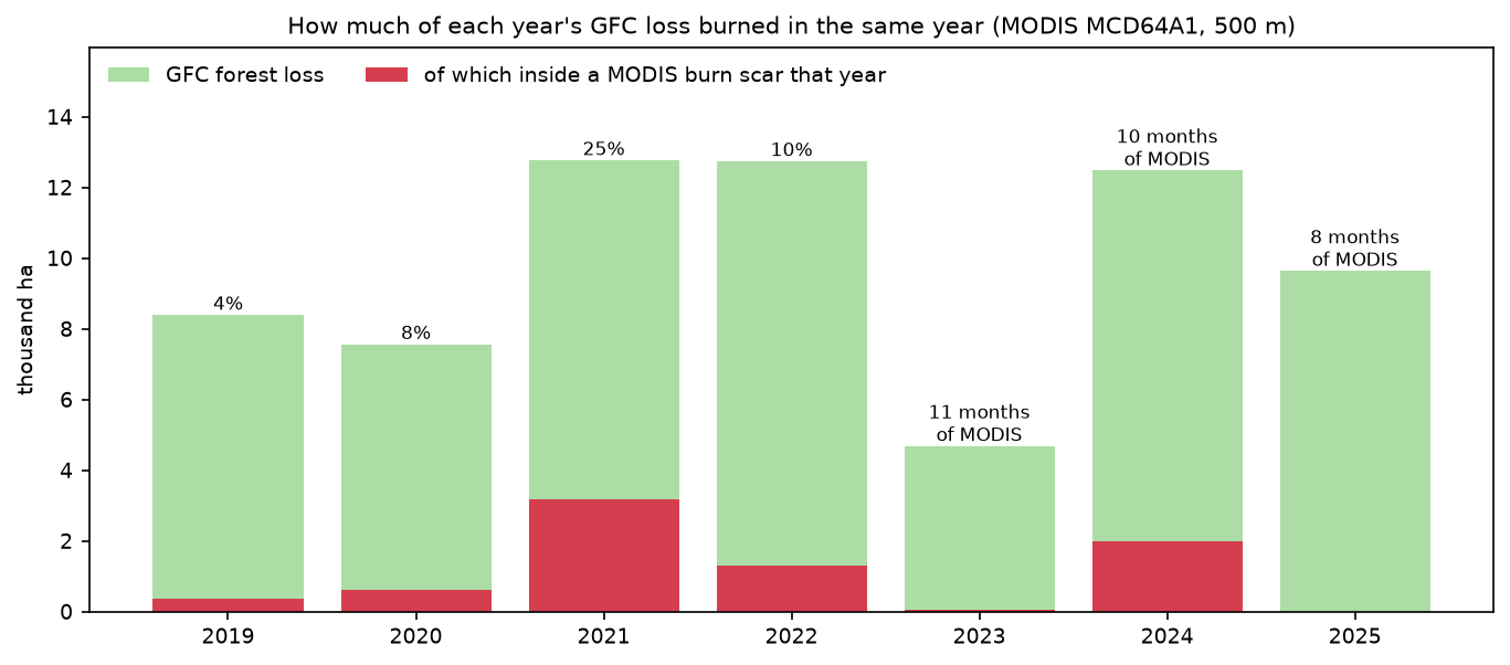
In the four complete years, 13.1% of GFC loss sat inside a same-year MODIS burn scar. That is a lower bound, for two reasons. MODIS misses small fires at 500 m, and many clearings are burned the year after they are cut. Even so, it shows that a real share of “forest loss” here involves fire.
The archive has gaps. 2023 lacks September, 2024 lacks July and November, and 2025 lacks May and August to October, which are the main burning months. The zero for 2025 therefore says nothing about 2025 fires. The script prints the months it found so that a gap like this cannot pass unnoticed.
Limitations and honest caveats
- Loss is not deforestation. GFC records any stand-replacing loss of canopy taller than 5 m. That includes clearing for pasture, which is permanent deforestation, but also fire, windthrow, river migration and the harvest of timber plantations, which will regrow. In Rondônia most loss is conversion to pasture. In Indonesian or Brazilian plantation landscapes a large share is harvest and replanting. Global Forest Watch publishes a separate “drivers of tree cover loss” layer for this reason.
- The method changed, and not for every year. In v1.13 the authors reprocessed 2011 onwards with Landsat 8 (from 2013) and Landsat 9 (from 2022), better training data and new features, which improves the detection of fire, smallholder clearing, selective logging and plantation clearing. Years 2001–2010 still use the old method. A jump across 2010/2011 may be partly an artefact, and figures from an older version for the same area will differ. A v2.0 is planned.
- Pixel counts are not unbiased area estimates. Even with correct pixel areas, the map has omission and commission errors. The GFC user notes recommend sample-based area estimation (for example, following Olofsson et al., 2014) for definitive figures, and a 3-year moving average for trends.
- No regrowth after 2012. The
gainlayer only covers 2000–2012, andlossyearrecords only the first loss. A pixel cleared in 2005 that regrew and was cleared again in 2021 still shows 2005, so loss after 2012 on regrown land is missed. - “Forest” depends on the threshold. Here it barely matters, but in drier or more open landscapes 10%, 30% and 50% canopy can give very different answers. GFC also counts plantations and tall shrubs as tree cover.
- The imagery checks are small. The NBR and MODIS checks cover one 13 km window and seven years. They test the timing and the fire share; they are not a formal accuracy assessment.
Frequently asked questions
How do I download Hansen Global Forest Change data in Python?
You don’t need to download it in advance. The tiles are public GeoTIFFs at https://storage.googleapis.com/earthenginepartners-hansen/GFC-2025-v1.13/Hansen_GFC-2025-v1.13_<layer>_<tile>.tif, where the tile is named after its north-west corner, such as 10S_070W. Open them with rasterio.open("/vsicurl/" + url) and read a window with rasterio.windows.from_bounds. Only the bytes for that window are transferred. The same layers are also in the Google Earth Engine data catalogue, if you prefer to work there.
What is the difference between tree cover loss and deforestation?
Tree cover loss is any removal of canopy, whatever the cause and whether or not the trees grow back. Deforestation is the permanent conversion of natural forest to another land use, such as pasture, cropland or towns. Fire, logging and plantation harvest all count as loss without necessarily being deforestation. To separate them, combine GFC with a drivers dataset, land-cover maps such as MapBiomas, or a later check of whether the forest returned.
Why does my GFC forest loss area differ from Global Forest Watch?
The usual causes are the canopy threshold (GFW defaults to 30%), the pixel area calculation (GFW uses true areas, so count × 0.09 will be too high), the version (each annual version reprocesses some years), and the boundary used. GFW statistics for administrative areas also apply its own masks, such as primary forest or plantations, in some views.
Can I detect deforestation in near real time?
GFC is annual and appears a few months after the year ends. For weekly alerts, use the GLAD Landsat alerts, the GLAD-S2 Sentinel-2 alerts or the RADD radar alerts on Global Forest Watch. In Brazil, INPE’s DETER system issues daily alerts. You can build a simple detector yourself from the NBR time series in Step 5, but clouds in the wet season are the main obstacle, which is why the RADD alerts use Sentinel-1 radar.
What canopy threshold should I use for forest?
30% is the most common choice and the Global Forest Watch default. Use the threshold in your country’s official forest definition if there is one; many follow the FAO definition of at least 10% canopy over 0.5 ha with trees taller than 5 m. Whatever you choose, report it, and test a few values as in Step 3.
Is GFC accurate enough for national statistics?
Not on its own. The authors and the IPCC good-practice guidance recommend using the map to stratify a random sample of reference points, interpreting those points visually, and estimating area and uncertainty from the sample. The map gives an excellent picture of where and when loss happened; the sample gives an unbiased number.
Next steps
- Separate pasture from other land cover after clearing with a random forest land cover classification of the 2025 Sentinel-2 image.
- Follow regrowth and degradation with a dense NDVI time series with odc-stac instead of one composite per year.
- Map the severity of the fires that show up as loss with burn severity mapping and dNBR.
- Outline individual clearings automatically with Segment Anything on satellite imagery.
- New to STAC? Start with measuring Lake Mead’s shoreline with Sentinel-2 and STAC.
- For a very different kind of spatial pattern analysis, see our hot spot analysis with Getis-Ord Gi* in Python. The same Gi* approach can find clusters of forest loss on a hexagon grid.
Data and licences
- Global Forest Change v1.13: Hansen, M. C., Potapov, P. V., Moore, R., Hancher, M., Turubanova, S. A., Tyukavina, A., Thau, D., Stehman, S. V., Goetz, S. J., Loveland, T. R., Kommareddy, A., Egorov, A., Chini, L., Justice, C. O. and Townshend, J. R. G. (2013), “High-Resolution Global Maps of 21st-Century Forest Cover Change”, Science 342: 850–853. Data available online from the Global Forest Change 2000–2025 site. Source: Hansen/UMD/Google/USGS/NASA, licensed under CC BY 4.0. Read from Google Cloud Storage on 19 October 2026.
- Sentinel-2 L2A: contains modified Copernicus Sentinel data 2017–2025, processed by ESA. Landsat 7 Collection 2 Level-2: courtesy of the U.S. Geological Survey. MODIS MCD64A1 v6.1: Giglio, L., Justice, C., Boschetti, L. and Roy, D., NASA LP DAAC. All accessed through the Microsoft Planetary Computer on 19 October 2026.
- Further reading: Olofsson, P. et al. (2014), “Good practices for estimating area and assessing accuracy of land change”, Remote Sensing of Environment 148: 42–57; Curtis, P. G. et al. (2018), “Classifying drivers of global forest loss”, Science 361: 1108–1111.
- Code:
deforestation_gfc.py, tested with Python 3.12.0, rasterio 1.5.2, numpy 2.5.4, pandas 3.0.6, pyproj 3.8.0, shapely 2.2.0, pystac-client 0.9.0, planetary-computer 1.0.0 and matplotlib 3.11.2.
Key terms
- Global Forest Change (GFC)
- The Hansen/UMD/Google/USGS/NASA global dataset of tree cover in 2000, annual tree cover loss since 2001 and gain from 2000 to 2012, made from Landsat at 0.00025° resolution. Global Forest Watch shows the same data.
- Tree cover loss
- In GFC, a stand-replacing disturbance: the complete removal of tree canopy at the scale of a Landsat pixel, for any reason. It is not the same as deforestation, which means a permanent change to another land use.
- Canopy threshold
- The percentage of tree canopy cover in 2000 above which a pixel counts as forest. Global Forest Watch defaults to 30%; results depend on the choice.
- lossyear
- The GFC layer that holds the year of loss as 1–25 for 2001–2025, with 0 for no loss detected.
- NBR
- Normalised Burn Ratio, (NIR − SWIR2) / (NIR + SWIR2). It is high over dense forest and drops sharply when canopy is cleared or burned.
- Pixel area on the ellipsoid
- The true ground area of a latitude/longitude pixel. Its east–west width shrinks with the cosine of latitude, so a fixed-degree pixel covers less ground towards the poles.
Data for this tutorial
- Hansen Global Forest Change · Tree cover 2000 and annual loss 2001–2025, v1.13, 10° × 10° GeoTIFF tiles
- Global Forest Watch · The same loss data in a web map, with country and subnational statistics
- Microsoft Planetary Computer · Sentinel-2 L2A, Landsat Collection 2 and MODIS MCD64A1 via STAC
- Landsat missions · The archive that GFC is built from, back to the 1980s
Licences and formats for each source are listed in the GIS data sources catalogue.