ERA5 in Python with xarray: mapping the July 2022 UK heatwave

Short answer: to use ERA5 in Python without a Copernicus account, open Google’s public ARCO-ERA5 Zarr store with xr.open_zarr("gs://gcp-public-data-arco-era5/ar/full_37-1h-0p25deg-chunk-1.zarr-v3", chunks=None, storage_options={"token": "anon"}). Select a variable, a time range and a lat/lon box with .sel(), then call .load() to download only those chunks. For GIS work, add a CRS with rioxarray, clip with .rio.clip(), average with cos(latitude) weights, and write a GeoTIFF with .rio.to_raster(..., driver="COG").

On 19 July 2022 the UK passed 40 °C for the first time on record: 40.3 °C at Coningsby in Lincolnshire, and 40.2 °C at Heathrow. In this tutorial we use ERA5, the most widely used climate reanalysis, to put that day in context. We compare it with every July day of the 1991–2020 standard period, map where it broke the 30-year record, and check how well a 0.25° model grid matches real thermometers.

You will learn how to:

1. open ERA5 from two free cloud Zarr stores (no CDS API key), and why their chunking decides which one to use;
2. turn hourly maximum temperature into daily Tmax correctly;
3. clip a lat/lon grid to a country polygon, and choose between cell centres, touching cells and the land-sea mask;
4. compute area-weighted means with cos(latitude);
5. map anomalies against a 1991–2020 climatology and export them as a Cloud Optimised GeoTIFF;
6. compare grid cells with Met Office station records, and correct for height and coastlines.

All outputs below are real results from era5_uk_heatwave.py, run on 21 October 2026 with Python 3.12, xarray 2026.9.0, zarr 3.4.1 and rioxarray 0.23.0.

What ERA5 is, and where to get it without a login

ERA5 is produced by ECMWF for the Copernicus Climate Change Service (C3S). A weather-forecast model is rerun for every hour since 1940, and at each step it is nudged towards millions of observations from weather stations, balloons, aircraft, ships and satellites. The result is a complete, consistent grid with no gaps: hourly, global, 0.25° (about 28 km north–south), with hundreds of variables at the surface and on 37 pressure levels. That makes it the default dataset for “what was the weather like here, then?” questions where there are no observations, and for climate baselines.

The official route is the Copernicus Climate Data Store (CDS) API, which needs an account and a queue. Two public copies need neither:

The layout matters more than anything else. Reading 30 Julys for the UK from ARCO means fetching 22,320 global chunks (about 52 GB) to keep 0.1% of each. From the Planetary Computer, the same request touches one chunk per month. So we use ARCO for July 2022 and the Planetary Computer for the 1991–2020 climatology, and check that the two agree.

Step 1: open ARCO-ERA5 lazily

xr.open_zarr reads only the metadata. Nothing is downloaded until you call .load() or .values:

ARCO = "gs://gcp-public-data-arco-era5/ar/full_37-1h-0p25deg-chunk-1.zarr-v3"
LON, LAT = (-8.75, 2.0), (61.0, 49.75)  # UK box; latitude runs north to south in ERA5

arco = xr.open_zarr(ARCO, chunks=None, storage_options={"token": "anon"})
mx2t = arco["maximum_2m_temperature_since_previous_post_processing"]

opened in 1.9 s: 273 variables, dims {'time': 1323648, 'latitude': 721, 'longitude': 1440, 'level': 37}
valid ERA5 data: 1940-01-01 to 2026-06-30 (ERA5T, preliminary, to 2026-10-15)
mx2t: Maximum temperature at 2 metres since previous post-processing [K], chunks (1, 721, 1440), 5.5 TB if loaded

storage_options={"token": "anon"} tells gcsfs to read the public bucket without Google credentials. chunks=None keeps the arrays lazy without building a Dask graph; with chunks={}, Dask would plan 1.3 million tasks per variable before doing anything.

Note the two dates. Data up to the end of June 2026 is final ERA5; the last few months are ERA5T, a preliminary version released about five days behind real time that is occasionally revised.

Step 2: hourly maxima to daily Tmax

We want the daily maximum temperature (Tmax), the quantity that weather stations report. ERA5 does not store Tmax directly. It stores mx2t, the highest 2 m temperature during the previous hour, so the value stamped 13:00 covers 12:00–13:00. Shift the time stamps back by an hour before taking the daily maximum, or each “day” will include the first hour of the next day:

def to_uk(da):
    """Convert 0..360 longitudes to -180..180 and cut out the UK box (still lazy)."""
    da = da.rename({k: v for k, v in {"lat": "latitude", "lon": "longitude"}.items() if k in da.dims})
    lon = da["longitude"]
    da = da.assign_coords(longitude=xr.where(lon > 180, lon - 360, lon)).sortby("longitude")
    return da.sel(longitude=slice(*LON), latitude=slice(*LAT))


def daily_max(hourly):
    """mx2t at hh:00 is the maximum over the previous hour, so shift by 1 h before taking the daily max."""
    shifted = hourly.assign_coords(time=hourly["time"] - np.timedelta64(1, "h"))
    return shifted.resample(time="1D").max()


hourly = to_uk(mx2t).sel(time=slice("2022-07-01T01", "2022-08-01T00")).load() - 273.15
tmax22 = daily_max(hourly)

ERA5 longitudes run from 0 to 360°, so the UK straddles the seam at 0°. to_uk relabels them as −180 to 180 and sorts, and only then slices the box. Latitude runs from north to south, so the slice is slice(61.0, 49.75), high to low.

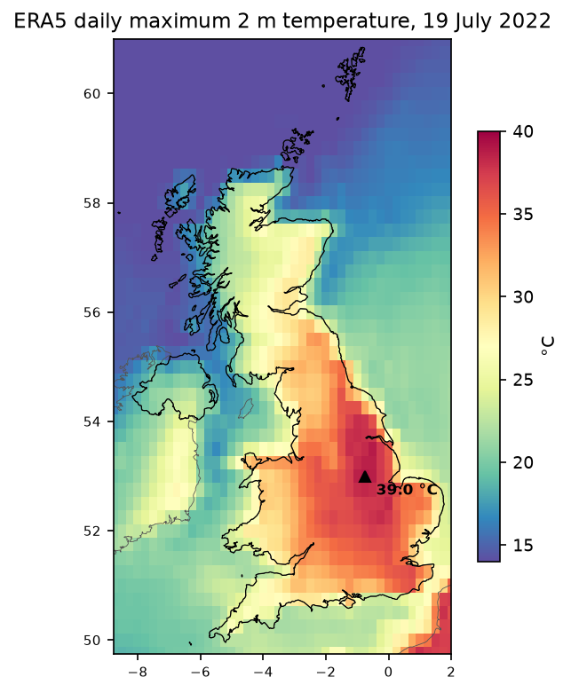
downloaded 744 hourly UK grids (744, 46, 44) in 51 s
daily Tmax grid: {'time': 31, 'latitude': 46, 'longitude': 44}; -8.75..2.0 E, 49.75..61.0 N
hottest ERA5 cell on 19 Jul 2022: 39.0 °C at 53.00 N, -0.75 E

The hottest ERA5 cell is in Lincolnshire, about 40 km west of Coningsby, where the UK record of 40.3 °C was set. ERA5 gets the place right and the peak about right for a 28 km cell.

Step 3: a 1991–2020 climatology from the Planetary Computer

The Planetary Computer catalogues its ERA5 copy in STAC, with one item per month and kind (an for analysis, fc for forecast variables such as maxima). Each asset carries the xarray:open_kwargs needed to open it:

catalog = pystac_client.Client.open("https://planetarycomputer.microsoft.com/api/stac/v1",
                                    modifier=planetary_computer.sign_inplace)
name = "air_temperature_at_2_metres_1hour_Maximum"
years = []
for year in range(1991, 2021):
    item = next(catalog.search(collections=["era5-pds"], datetime=f"{year}-07",
                               query={"era5:kind": {"eq": "fc"}}).items())
    asset = item.assets[name]
    ds = xr.open_dataset(asset.href, chunks={}, **asset.extra_fields["xarray:open_kwargs"])
    hourly = to_uk(ds[name]).load() - 273.15
    years.append(daily_max(hourly).sel(time=f"{year}-07"))
clim_daily = xr.concat(years, "time").rename("tmax")

The abfs:// URLs need the adlfs package installed. The variable names differ from ARCO and the coordinates are called lat and lon, which to_uk renames.

era5-pds-1991-07-fc: chunks {'time': 372, 'lat': 150, 'lon': 150}
downloaded 30 Julys in 72 s
climatology: 930 July days, 1991-2020
ARCO vs Planetary Computer, 15 Jul 2020 daily Tmax: max |diff| 0.032 °C

Thirty Julys in 72 seconds. The two copies agree to within 0.03 °C on a test day (they were produced and packed separately), so we can mix them safely. From the daily grids we build three fields:

clim_mean = clim_daily.mean("time")          # mean July daily maximum, 1991-2020
clim_record = clim_daily.max("time")         # highest July daily maximum, 1991-2020
hot = tmax22.sel(time="2022-07-19").squeeze(drop=True)
anom_month = tmax22.mean("time") - clim_mean
anom_19 = hot - clim_mean
above_record = hot - clim_record             # > 0 where 19 July beat every July day of 1991-2020

Step 4: clip to the UK polygon

ERA5 is a regular lat/lon grid, so to rioxarray it is just a raster in EPSG:4326. Tell it which dimensions are x and y, write the CRS, and clip with any polygon. We use the Natural Earth 1:10m country boundaries:

countries = gpd.read_file("ne_10m_admin_0_countries.zip")
uk = countries[countries["ADMIN"] == "United Kingdom"].to_crs(4326)


def georef(da):
    return da.rio.set_spatial_dims(x_dim="longitude", y_dim="latitude").rio.write_crs("EPSG:4326")


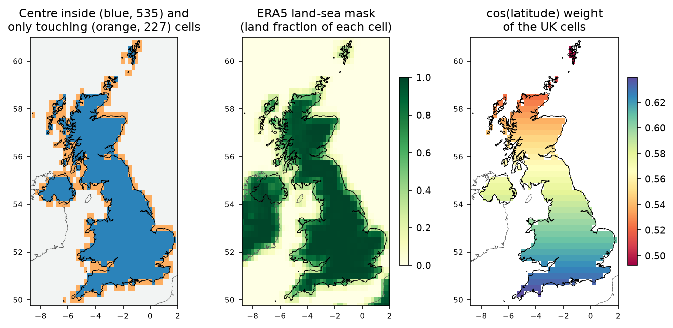
clip_centre = georef(clim_mean).rio.clip(uk.geometry, all_touched=False, drop=False)
clip_touch = georef(clim_mean).rio.clip(uk.geometry, all_touched=True, drop=False)
land = static["land_sea_mask"] > 0.5
inside = clip_centre.notnull()

grid transform: (0.25, 0.0, -8.875, 0.0, -0.25, 61.125)
cells with centre inside the UK: 535; touching the UK: 762; land-sea mask > 0.5 in box: 650
of the centre-inside cells, 503 are also land (lsm > 0.5)

The transform shows that rioxarray treats each value as a cell centred on its coordinate: the first cell spans −8.875 to −8.625°. That is the right reading of ERA5. The choice of clip rule changes the answer noticeably at this resolution:

• Centre inside (all_touched=False, the default) keeps 535 cells. Use it for averages.
• All touched keeps 762 cells, 42% more, including many that are mostly sea. Use it when you must not lose any coast, for example when exporting a map to clip again later.
• The ERA5 land-sea mask (land_sea_mask, the land fraction of each cell) is the model’s own idea of the coast. Combine it with the polygon when you need land-only values.

Step 5: area-weighted UK means

A 0.25° × 0.25° cell gets narrower towards the poles: its east–west width is proportional to the cosine of the latitude. A plain .mean() over the grid therefore gives Shetland too much weight. xarray’s .weighted() fixes that:

weights = np.cos(np.deg2rad(clim_mean.latitude))


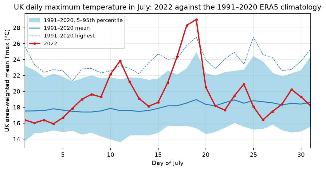
def uk_mean(da, weighted=True):
    da = da.where(inside)
    return da.weighted(weights).mean(("latitude", "longitude")) if weighted else da.mean(("latitude", "longitude"))

cos(lat) weight: 0.485 at 61.00 N, 0.646 at 49.75 N
cell area: 499 km² in the south, 375 km² in the north; UK cells total 241,786 km²
UK mean July daily Tmax 1991-2020: 18.07 °C (unweighted 17.97)
UK mean July daily Tmax 2022:      19.61 °C, anomaly +1.54 °C
  19 Jul 2022: UK-mean Tmax 29.0 °C, 1991-2020 mean for the day 19.0, highest of the 30 years 26.8
  18 Jul 2022: UK-mean Tmax 28.3 °C, 1991-2020 mean for the day 18.5, highest of the 30 years 25.8
  17 Jul 2022: UK-mean Tmax 24.4 °C, 1991-2020 mean for the day 18.2, highest of the 30 years 24.1
warmest UK-mean July day in 1991-2020: 26.8 °C on 19 Jul 2006
19 Jul 2022 anomaly: mean +11.0 °C, max +18.1 °C; 61% of UK area above its 1991-2020 July record

Weighting moves the UK July mean by only 0.1 °C here, because the UK spans just 11° of latitude and the weights only range from 0.49 to 0.65. Over larger latitude ranges, such as Europe or a hemisphere, it matters far more. The 535 cells add up to 241,786 km², close to the UK’s real area of about 243,000 km², which is a useful check of the clip.

The time series puts 19 July in context. The UK as a whole averaged a daily maximum of 29.0 °C, 10 °C above normal for the date and 2.2 °C above the warmest UK-wide July day of the previous 30 years (19 July 2006).

Step 6: anomaly maps and a Cloud Optimised GeoTIFF

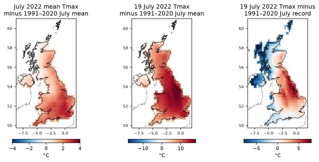
The right-hand map is the most telling: across 61% of the UK by area, 19 July was hotter than any July day of 1991–2020 in that cell. The record-breaking zone runs from London to the Scottish border, along the east side of the Pennines, which matches where the Met Office reported new station records.

To use these fields in QGIS or ArcGIS Pro, write them as a multi-band GeoTIFF. Rasterio’s COG driver writes a Cloud Optimised GeoTIFF directly:

stack = xr.concat([anom_month, anom_19, above_record], dim="band").assign_coords(band=[1, 2, 3])
stack = georef(stack.astype("float32").where(clip_touch.notnull())).rio.write_nodata(np.nan)
stack.attrs = {"long_name": ("July 2022 mean Tmax anomaly", "19 July 2022 Tmax anomaly",
                             "19 July 2022 Tmax minus 1991-2020 July record"), "units": "degC"}
stack.rio.to_raster("era5_uk_tmax_anomaly_2022-07.tif", driver="COG", compress="DEFLATE", predictor=3)

era5_uk_tmax_anomaly_2022-07.tif: GTiff, 3 bands float32, 44 x 46, EPSG:4326, res (0.25, 0.25), layout COG, 14 KB
bounds (-8.875, 49.625, 2.125, 61.125); band 2 at Heathrow: 14.1 °C
band descriptions: ('July 2022 mean Tmax anomaly', '19 July 2022 Tmax anomaly', '19 July 2022 Tmax minus 1991-2020 July record')

Three things to notice:

• Reading the file back, rasterio reports the driver as GTiff with LAYOUT=COG in its image-structure metadata. A COG is a GeoTIFF, so any GIS can open it; the layout tag is how you confirm it was written as one.
• We exported with the all-touched mask, so coastal cells are kept and a user can clip again with a finer coastline.
• predictor=3 is the floating-point predictor, which makes DEFLATE compress float data much better. Setting long_name as a tuple fills the band descriptions, so the bands are labelled in QGIS.

Step 7: compare ERA5 with Met Office stations

A reanalysis is a model, so it is worth checking against thermometers. The Met Office publishes monthly records for 37 long-running stations as plain text, free of charge, with mean daily maximum temperature (tmax) and the station’s position and height:

MO = "https://www.metoffice.gov.uk/pub/data/weather/uk/climate/stationdata/{}data.txt"
txt = requests.get(MO.format("heathrow"), timeout=60).text
lat, lon = map(float, re.search(r"Lat\s*([-\d.]+)\s*,?\s*Lon\s*([-\d.]+)", txt).groups())
alt = float(re.search(r"(-?[\d.]+)\s*m(?:etres)?\s*amsl", txt).group(1))
# then keep rows where month == 7; strip '*' (estimated) and '#' (automatic station) flags

Two corrections make the comparison fairer. First, the ERA5 cell’s surface height (geopotential_at_surface / 9.80665) is the average over 28 km and can differ from the station height by hundreds of metres in hills; a standard lapse rate of 6.5 °C per km adjusts for that. Second, a coastal station often falls in a cell that is mostly sea, where the model’s air is cooler in summer; using the nearest land cell (land-sea mask > 0.5) avoids that:

z_era5 = static["geopotential_at_surface"] / 9.80665
lapse = lambda p: 0.0065 * (at(z_era5, p) - meta["alt"].values)   # ERA5 cell higher -> ERA5 too cool
cmp["era5_2022"] = at(tmax22.mean("time"), pts)
cmp["era5_2022_lapse"] = cmp["era5_2022"] + lapse(pts)
cmp["era5_2022_land"] = at(tmax22.mean("time"), land_pts) + lapse(land_pts)

Here pts are the station coordinates, land_pts the centre of the nearest land cell to each station, and at() is a vectorised .sel(..., method="nearest"). See the full script for those helpers.

37 stations, 3244 July means; 31 stations reported July 2022
6 of 37 stations are nearer a sea or coastal cell than the centre of a land cell
July 2022 mean Tmax, ERA5 vs station
  nearest cell:                        n=31, bias -2.38 °C, MAE 2.38 °C, r=0.93
  + 6.5 °C/km lapse-rate correction:   n=31, bias -2.23 °C, MAE 2.23 °C, r=0.94
  nearest land cell + lapse rate:      n=31, bias -1.58 °C, MAE 1.70 °C, r=0.94
1991-2020 July mean Tmax, nearest land cell + lapse rate: n=31, bias -1.40 °C, MAE 1.46 °C, r=0.93
                     alt  era_z  lsm  obs_2022  era5_2022  era5_2022_land  diff_2022
station
Hurn                10.0   23.0  0.6      24.7       20.9            21.0       -3.7
Whitby Coastguard   60.0   53.0  0.3      22.8       17.1            19.5       -3.3
Leuchars            10.0   56.0  0.7      22.0       18.4            18.7       -3.3
Aberporth          133.0   53.0  0.3      19.8       18.6            19.9        0.1
Lerwick             82.0   16.0  0.4      14.2       12.3            14.7        0.5
Camborne            87.0   33.0  0.4      20.8       20.8            22.0        1.2
Heathrow July means 1991-2020: r=0.99 between station and ERA5 year to year
Heathrow 19 Jul 2022: ERA5 cell 35.2 °C (the station recorded 40.2 °C that day)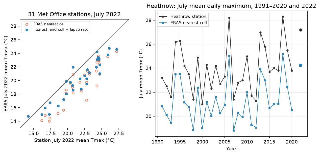

What this tells us:

• ERA5 is too cool for summer daytime maxima in the UK: by 1.6 °C on average in July 2022 after both corrections, and by 1.4 °C over 1991–2020. This is a known ERA5 bias. Part of it is resolution (a 28 km cell blends towns, fields, hills and sea), and part of it is the model’s surface physics.
• The land-cell correction matters more than the height correction at these mostly low-lying stations. At Whitby it reduces the error from 5.7 to 3.3 °C.
• Year-to-year variation is excellent (r = 0.99 at Heathrow). ERA5 anomalies are much more reliable than its absolute values, which is why we mapped anomalies.
• Extremes are smoothed. On 19 July the Heathrow cell reached 35.2 °C, 5 °C below the station’s 40.2 °C. Heathrow sits in an urban heat island that a 28 km cell cannot resolve. Never quote an ERA5 cell value as “the temperature at” a town on a record day.

Limitations

• Resolution. At 0.25° each cell is about 28 × 17 km in the UK. Islands, coasts, cities and valleys are blended. For UK work at 1 to 5 km, the Met Office’s HadUK-Grid (station-based) is the reference; ERA5-Land offers 0.1° but only for land variables.
• Bias in Tmax. As measured above, ERA5 underestimates UK summer maxima by 1 to 2 °C on average and by more on extreme days. Use anomalies, or bias-correct against stations, before drawing conclusions about absolute values.
• ERA5T. The last two or three months in ARCO-ERA5 are preliminary and can be revised; check valid_time_stop before using recent data.
• Different day definitions. Our ERA5 days run midnight to midnight UTC. Met Office climatological days run 09:00 to 09:00 UTC. That matters little for monthly means but can shift daily extremes.
• Planetary Computer coverage. The era5-pds copy ends in December 2020. For later baselines, use ARCO-ERA5 with patience, or the NSF NCAR ERA5 copy on AWS (s3://nsf-ncar-era5), which is chunked by region and month.
• Station gaps. Six of the 37 stations did not report July 2022 in this archive, and the comparison uses monthly means, not daily values.

Frequently asked questions

Can I download ERA5 in Python without a CDS account?

Yes. Google’s ARCO-ERA5 (gs://gcp-public-data-arco-era5) and the Microsoft Planetary Computer’s era5-pds collection are public and open with xarray and no credentials, as in this tutorial. NSF NCAR also publishes ERA5 as netCDF on AWS (s3://nsf-ncar-era5). The CDS API remains the official route and the only one for some less common variables, but it needs an account and requests can queue for hours.

How do I get daily maximum temperature from ERA5?

Use the mx2t variable (maximum_2m_temperature_since_previous_post_processing in ARCO-ERA5), shift the time stamps back by one hour because each value covers the previous hour, and take .resample(time="1D").max(). Taking the daily maximum of the hourly 2m_temperature instead underestimates Tmax slightly, because the peak usually falls between hours.

Why do I need to weight by cos(latitude)?

On a regular lat/lon grid, cells get narrower towards the poles: a 0.25° cell covers 499 km² at 50° N but 375 km² at 61° N. An unweighted mean counts each cell equally and so over-represents high latitudes. da.weighted(np.cos(np.deg2rad(da.latitude))).mean(...) gives each cell its true share of the area.

Is ERA5 accurate enough to compare with weather stations?

For anomalies and year-to-year changes, yes: July means at Heathrow correlate at r = 0.99. For absolute values, expect biases of 1 to 2 °C in UK summer maxima, and much larger misses on extreme days and in towns, hills and coasts, because each cell averages 400 to 500 km². Correct for height, use the nearest land cell for coastal stations, and compare like with like (monthly with monthly).

How do I convert ERA5 to GeoTIFF?

Use rioxarray: set the spatial dimensions with .rio.set_spatial_dims(x_dim="longitude", y_dim="latitude"), write the CRS with .rio.write_crs("EPSG:4326"), and save with .rio.to_raster("out.tif", driver="COG"). Convert longitudes from 0–360 to −180–180 first if your region crosses the prime meridian.

Next steps

• Swap the variable: total precipitation (total_precipitation) for drought and rainfall anomalies, or 10 m wind for storm footprints. The clipping, weighting and export steps do not change.
• Compare a reanalysis air temperature with what satellites see at the ground in Land surface temperature from Landsat in Python.
• Interpolate the station records yourself and compare the surface with ERA5 using Kriging spatial interpolation in Python.
• Find statistically significant hot spots in the anomaly grid with Hot spot analysis with Getis-Ord Gi* in Python.
• Combine ERA5 wind and boundary-layer height with satellite air-quality data in Sentinel-5P NO₂ air pollution in Python.
• Learn more about streaming raster data with rioxarray in Terrain analysis in Python with rasterio and rioxarray.

Data and licences

• ERA5: Hersbach, H. et al. (2020), “The ERA5 global reanalysis”, Quarterly Journal of the Royal Meteorological Society 146(730). Contains modified Copernicus Climate Change Service information 2026; neither the European Commission nor ECMWF is responsible for any use of this information. Accessed via ARCO-ERA5 (Carver and Merose, 2023) on Google Cloud and the Microsoft Planetary Computer on 21 October 2026.
• Met Office historic station data: © Crown copyright, Met Office, from metoffice.gov.uk, licensed under the Open Government Licence v3.0. Some recent values are provisional.
• Country boundaries: Natural Earth 1:10m Admin 0 countries, public domain.
• Code: era5_uk_heatwave.py, tested with Python 3.12.0, xarray 2026.9.0, zarr 3.4.1, gcsfs 2026.10.1, adlfs 2026.8.0, rioxarray 0.23.0, rasterio 1.5.2 and geopandas 1.2.0.