Glacier velocity in Python with NASA ITS_LIVE: Jakobshavn Isbræ, 1985–2025

Short answer: to get glacier velocity in Python, use NASA’s ITS_LIVE data. Find the datacube that covers your glacier in the public GeoJSON catalogue, then open it with xr.open_dataset(zarr_url, engine="zarr"). No login, API key or download is needed, because the Zarr stores sit in a public AWS S3 bucket. The annual composites give clean maps (v, vx, vy) and a 2014–2024 climatology (v0). The image-pair datacube gives every individual velocity measurement since 1984, which you filter by time separation (date_dt) and error (v_error) before building time series.

Jakobshavn Isbræ (Sermeq Kujalleq in Greenlandic) drains about 6.5% of the Greenland Ice Sheet into Disko Bay through the Ilulissat Icefjord, a UNESCO World Heritage Site. It is one of the fastest glaciers on Earth. After its floating tongue broke up between 1998 and 2003, it roughly doubled in speed (Joughin et al., 2004). It then slowed sharply in 2016–2018, when cooler ocean water reached the fjord (Khazendar et al., 2019). That history makes it an ideal test case: the signal is large, well documented and visible at every timescale from months to decades.

You will learn how to:

1. find and open the right ITS_LIVE datacube from the public catalogue, lazily, with xarray;
2. map surface speed from the annual composites and the 2014–2024 climatology;
3. trace a flowline by integrating the velocity vectors, and extract speed profiles along it from 1985 to 2025;
4. pull the image-pair time series at points on the flowline and filter it by time separation, error and a rolling-median test;
5. measure the seasonal cycle and the multi-year change, and check them against the composites;
6. compute strain rates and plot flow direction with a quiver plot.

All outputs below are real results from glacier_velocity_its_live.py, run on 21 October 2026 with Python 3.12, xarray 2026.9.0, zarr 3.4.1 and scipy 1.18.1.

How ITS_LIVE measures glacier velocity

ITS_LIVE measures velocity by feature tracking. Take two images of the same glacier a few days or weeks apart. Crevasses, rifts, debris bands and snow dunes move with the ice. For each small window (a chip) of the first image, the autoRIFT algorithm (Lei et al., 2021) searches the second image for the best match by normalised cross-correlation, and refines it to a fraction of a pixel. The offset in metres, divided by the time between the images, is the surface velocity. Repeating this on a grid gives a velocity field with an x and a y component.

ITS_LIVE runs this on every suitable pair from Landsat 4–9 and Sentinel-2 (optical, which needs daylight and no cloud) and Sentinel-1 (radar amplitude, which works through cloud and in the polar night). Each pair becomes one layer in a datacube, labelled by its mid_date (half way between the two images), with its time separation date_dt in days, error estimates (v_error) and the sensors used. That has three consequences that shape the rest of this tutorial:

• Every measurement is an average over its time separation. A 12-day Sentinel-1 pair sees the summer speed-up; a 365-day Landsat pair averages over it.
• Matching can fail. If the ice has changed too much (fast flow, melt, fresh snow) or the offset is larger than the search window, autoRIFT may lock onto stable features and report a speed that is far too low. Long pairs on fast ice are the classic case.
• Errors differ by sensor and by pair. Filtering on date_dt and v_error is not optional.

Step 1: find the datacube that covers the glacier

ITS_LIVE splits the world into 100 km × 100 km Zarr datacubes in local projections: polar stereographic (EPSG:3413) for Greenland. A GeoJSON catalogue lists every cube’s footprint and URL, so finding the right one is a point-in-polygon test with geopandas.

import geopandas as gpd
import requests
import xarray as xr
from shapely.geometry import Point

LON, LAT = -49.14, 69.10            # a point on the main trunk of Jakobshavn Isbrae, ~25 km above the front
CATALOG = "https://its-live-data.s3.amazonaws.com/datacubes/catalog_v02.json"
cat_path = DATA / "catalog_v02.json"
if not cat_path.exists():
    cat_path.write_bytes(requests.get(CATALOG, timeout=300).content)
catalog = gpd.read_file(cat_path)
hit = catalog[catalog.contains(Point(LON, LAT))].iloc[0]
print(f"catalogue: {len(catalog)} datacubes")
print(f"cube:      {hit.zarr_url}")
print(f"composite: {hit.composite_zarr_url}")

cube = xr.open_dataset(hit.zarr_url, engine="zarr", chunks={})          # lazy: nothing downloaded yet
comp = xr.open_dataset(hit.composite_zarr_url, engine="zarr", chunks={})

catalogue: 3160 datacubes
cube:      https://its-live-data.s3.amazonaws.com/datacubes/v2-updated-october2024/N60W040/ITS_LIVE_vel_EPSG3413_G0120_X-150000_Y-2250000.zarr
composite: https://its-live-data.s3.amazonaws.com/composites/annual/v2-updated-september2025/N60W040/ITS_LIVE_velocity_EPSG3413_120m_X-150000_Y-2250000.zarr
EPSG:3413, 80568 image pairs
datacube: 80568 image pairs on a 833 x 833 grid of 120 m pixels, chunks (20000, 10, 10)
mid_date range: 1984-10-21 to 2025-05-28
composites: 42 annual mosaics, 1984-2025

chunks={} keeps everything lazy: opening the cube reads only its metadata. Note the chunk shape, (20000, 10, 10). Each chunk holds 20,000 dates for a 10 × 10 pixel block, so the cube is optimised for time series at a point: reading every image pair at one pixel touches only five chunks and took about a second. Reading a full map for one date would touch thousands of chunks. That is why maps come from the composites, which are chunked the other way.

Step 2: map glacier speed from the annual composites

The composite store has one mosaic per calendar year (v, vx, vy, v_error) and a fitted climatology for 2014–2024: the mean speed v0, the components vx0 and vy0, and the amplitude (v_amp) and phase (v_phase) of a seasonal sine wave. These are small enough to load whole.

v0 = comp.v0.load()                                  # 2014-2024 climatological speed (time intercept 2018-01-01)
vx0, vy0 = comp.vx0.load(), comp.vy0.load()
v_amp, v_phase = comp.v_amp.load(), comp.v_phase.load()
landice = comp.landice.load()
x, y = comp.x.values, comp.y.values
print(f"fastest climatological speed in the cube: {float(v0.max()):,.0f} m/yr")
print(f"pixels with v0 > 1 km/yr: {int((v0 > 1000).sum()):,} ({int((v0 > 1000).sum()) * 0.12 ** 2:,.0f} km2)")

fastest climatological speed in the cube: 15,195 m/yr
pixels with v0 > 1 km/yr: 41,503 (598 km2)

A logarithmic colour scale is essential: the ice sheet interior moves at tens of metres a year and the trunk at over 10,000.

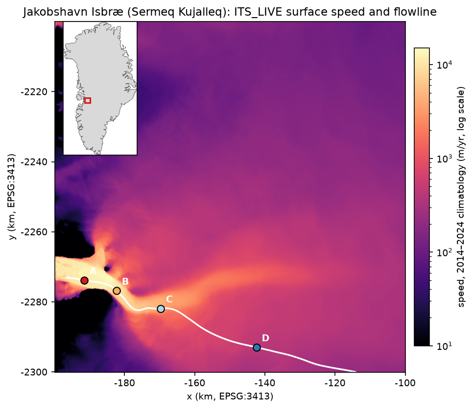
Annual maps show how much the glacier changes from year to year. 2013 was close to the peak of the post-2003 acceleration; 2017 was in the middle of the slowdown.

MAP_YEARS = [2013, 2017, 2024]
yr = {y_: comp.v.sel(time=f"{y_}-01-01").load() for y_ in MAP_YEARS}
im2 = axs[1, 1].imshow(yr[2017] - yr[2013], extent=ext, cmap="RdBu_r", norm=TwoSlopeNorm(0, -4000, 4000))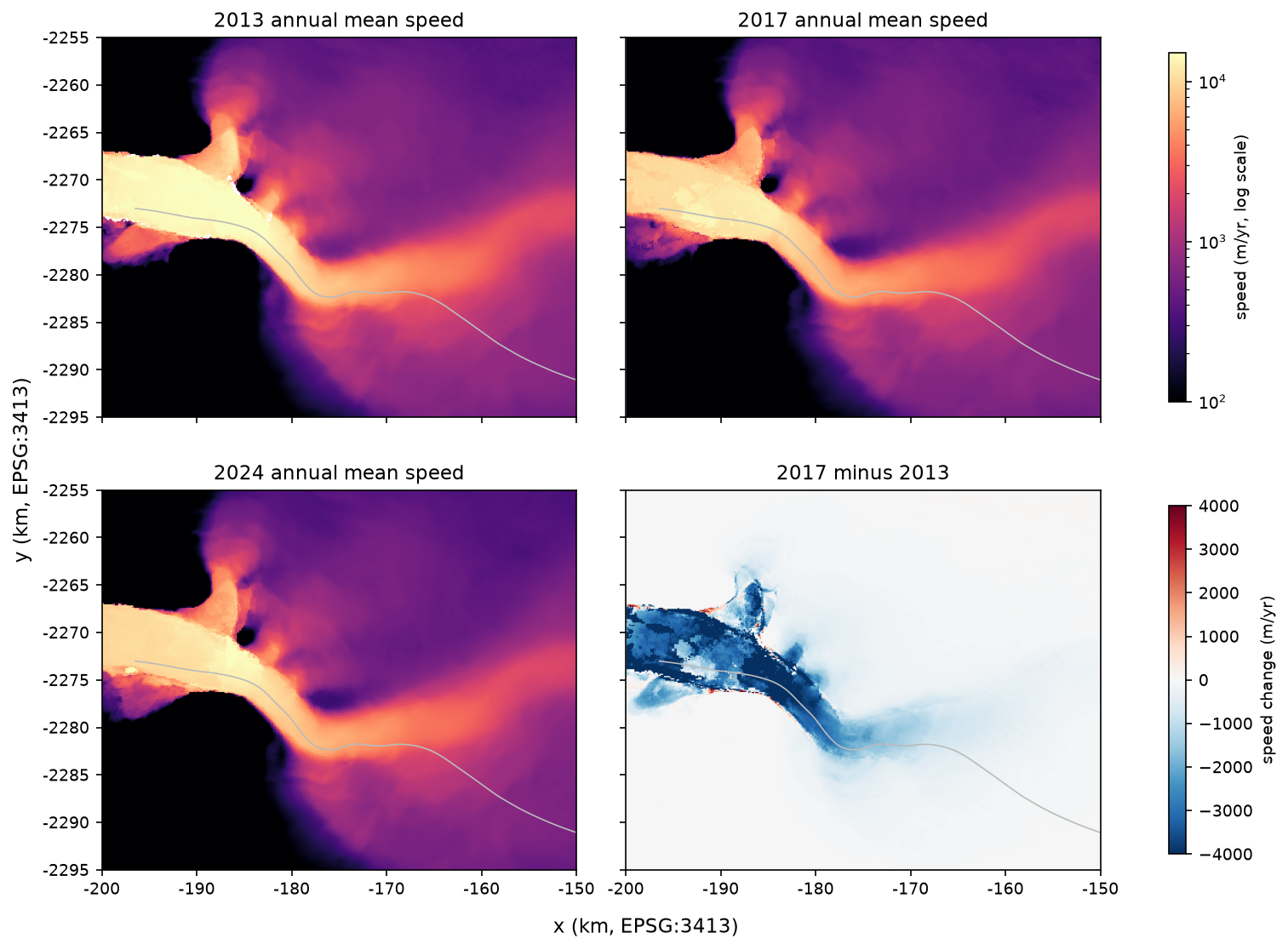

Step 3: trace a flowline and extract speed profiles

A flowline follows the ice from the ice sheet to the front. We trace it by stepping along the direction of the climatological velocity vectors with a fourth-order Runge–Kutta integrator: upstream until the ice slows below 200 m/yr or we leave the cube, and downstream until the ice reaches the end of the composite’s land-ice mask. Beyond the mask edge is the ice mélange in the fjord, which moves but is not glacier.

from scipy import ndimage
from scipy.interpolate import RegularGridInterpolator

# Smooth the vectors a little, then interpolate them anywhere on the grid.
valid = ndimage.gaussian_filter(np.isfinite(vx0.values).astype(float), 2)
sx = ndimage.gaussian_filter(np.nan_to_num(vx0.values), 2) / np.maximum(valid, 1e-6)
sy = ndimage.gaussian_filter(np.nan_to_num(vy0.values), 2) / np.maximum(valid, 1e-6)
sx[valid < 0.5] = np.nan
sy[valid < 0.5] = np.nan
grid = (y[::-1], x)                                   # RegularGridInterpolator needs ascending axes
ix = RegularGridInterpolator(grid, sx[::-1], bounds_error=False, fill_value=np.nan)
iy = RegularGridInterpolator(grid, sy[::-1], bounds_error=False, fill_value=np.nan)
spd = RegularGridInterpolator(grid, v0.values[::-1], bounds_error=False, fill_value=np.nan)


def unit(p):
    u_, v_ = ix([p[::-1]])[0], iy([p[::-1]])[0]
    n = np.hypot(u_, v_)
    return np.array([u_, v_]) / n if np.isfinite(n) and n > 0 else None


def trace(start, sign, step=120.0, max_km=150, min_speed=200.0):
    pts_ = [np.asarray(start, float)]
    for _ in range(int(max_km * 1000 / step)):
        p = pts_[-1]
        k1 = unit(p)
        k2 = unit(p + sign * step / 2 * k1) if k1 is not None else None
        k3 = unit(p + sign * step / 2 * k2) if k2 is not None else None
        k4 = unit(p + sign * step * k3) if k3 is not None else None
        if k4 is None:
            break
        q = p + sign * step / 6 * (k1 + 2 * k2 + 2 * k3 + k4)
        if not (x[0] < q[0] < x[-1] and y[-1] < q[1] < y[0]) or not spd([q[::-1]])[0] >= min_speed:
            break
        pts_.append(q)
    return np.array(pts_)


lon_to = Transformer.from_crs("EPSG:4326", f"EPSG:{hit.epsg}", always_xy=True)
seed = np.array(lon_to.transform(LON, LAT))
line = np.vstack([trace(seed, -1)[::-1], trace(seed, +1)[1:]])
# End the flowline where the static land-ice mask ends: beyond it is the ice melange in the fjord.
on_ice = landice.sel(x=xr.DataArray(line[:, 0]), y=xr.DataArray(line[:, 1]), method="nearest").values == 1
line = line[: np.flatnonzero(on_ice)[-1] + 1]

Where you put the seed matters. Jakobshavn has a northern and a southern branch that join about 15 km above the front. A seed on the lower trunk, traced upstream, follows whichever branch the vectors favour, so check the line on the map. Our seed, on the trunk about 25 km above the front, follows the main southern branch.

Then sample every annual composite along the line with vectorised (pointwise) indexing, and drop values whose error is more than 25% of the speed:

lx, ly = xr.DataArray(line[:, 0], dims="d"), xr.DataArray(line[:, 1], dims="d")
prof = comp.v.sel(x=lx, y=ly, method="nearest").load()
prof_err = comp.v_error.sel(x=lx, y=ly, method="nearest").load()
prof = prof.where(prof_err < 0.25 * prof)                # drop poorly constrained annual values

flowline: 743 vertices, 89.0 km long; ice-mask edge at x=-196465, y=-2273015; upstream end at x=-114215, y=-2299962
point A:  5 km upstream, x=-191493, y=-2273824, v0=11,810 m/yr
point B: 15 km upstream, x=-182234, y=-2276829, v0=10,223 m/yr
point C: 30 km upstream, x=-169666, y=-2281882, v0=3,829 m/yr
point D: 60 km upstream, x=-142347, y=-2292969, v0=438 m/yr

      A (5 km)  B (15 km)  C (30 km)  D (60 km)  max on line
year
1985    6208.0     5527.0     1871.0        NaN       6472.0
1995    5885.0     4435.0     1822.0        NaN       6028.0
2000   10143.0     7583.0     2605.0        NaN      10447.0
2003   14233.0    10616.0     3274.0      363.0      14790.0
2007   15276.0    10554.0     3530.0      376.0      15703.0
2013   14481.0    13767.0     4819.0      438.0      16721.0
2015   13355.0    12647.0     4663.0      455.0      15825.0
2017   13482.0     9451.0     3776.0      452.0      15230.0
2018   11263.0     7997.0     3385.0      431.0      12189.0
2019    9569.0    10523.0     3692.0      419.0      11479.0
2021   13731.0    13190.0     4919.0      429.0      15364.0
2022   10052.0    10866.0     4105.0      423.0      12365.0
2024   10489.0    10436.0     4032.0      420.0      13482.0
2025   11719.0    11291.0     4138.0      415.0      13597.0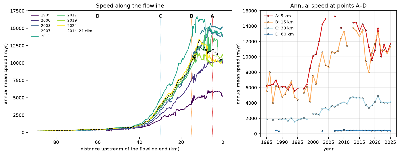

The profiles tell the story of the glacier. In 1995 the lower trunk moved at about 6 km/yr. After the floating tongue broke up, point A sped up to over 14 km/yr by 2003 and 15.3 km/yr by 2007, and the speed-up spread more than 30 km inland: point C went from 1,822 m/yr in 1995 to 4,819 m/yr in 2013. Between 2015 and 2019, point A slowed by 28%, from 13,355 to 9,569 m/yr, and it sped up again in 2021. Point D, 60 km inland, barely changed.

Step 4: image-pair time series and error filtering

For anything shorter than a year you need the image-pair datacube. Select the nearest pixel to each point and load the variables you need. This is where the time-first chunking pays off.

VARS = ["v", "v_error", "date_dt", "mission_img1", "satellite_img1"]
series = {}
for k, p in pts.items():
    s = cube[VARS].sel(x=p[0], y=p[1], method="nearest").load().to_dataframe()
    s = s.dropna(subset=["v"]).sort_index()              # mid_date is not sorted in the cube
    s["sensor"] = s.mission_img1.astype(str) + s.satellite_img1.astype(str)
    series[k] = s

point A: 2,320 image pairs with a value, 1985-03-21 to 2025-05-10
point B: 4,422 image pairs with a value, 1985-04-06 to 2025-05-22
point C: 5,304 image pairs with a value, 1985-03-29 to 2025-05-22
point D: 7,593 image pairs with a value, 1985-06-22 to 2025-05-22

The raw series are noisy. We apply three filters, to pairs from 2014 onwards (when Sentinel-1, Sentinel-2 and Landsat 8 give a dense record):

1. Time separation: keep pairs at most 48 days apart. They resolve the seasonal cycle, and they are where feature tracking works best on fast ice.
2. Error: keep pairs whose v_error is at most 15% of the speed.
3. Outliers: keep pairs within 3 median absolute deviations (MAD) of a centred 45-day rolling median, with a floor of 2% of the median.

def clean(s: pd.DataFrame, max_dt=48, max_rel_err=0.15, window="45D", n_mad=3.0) -> pd.DataFrame:
    """Flag short, well-constrained pairs whose speed is close to the local rolling median."""
    s = s[s.index >= "2014-01-01"].copy()
    s["keep_dt"] = s.date_dt <= max_dt
    s["keep_err"] = s.v_error <= max_rel_err * s.v
    s1 = s[s.keep_dt & s.keep_err]
    med = s1.v.rolling(window, center=True, min_periods=5).median()
    mad = (s1.v - med).abs().rolling(window, center=True, min_periods=5).median() * 1.4826
    ok = (s1.v - med).abs() <= n_mad * np.maximum(mad, 0.02 * med)
    s["keep_mad"] = False
    s.loc[s1.index[ok.values], "keep_mad"] = True
    s["keep"] = s.keep_dt & s.keep_err & s.keep_mad
    return s


filt = {k: clean(s) for k, s in series.items()}

   pairs since 2014  dt <= 48 d  + error <= 15%  + rolling MAD  kept %
A            1648.0      1493.0          1493.0         1267.0    76.9
B            3873.0      2870.0          2870.0         2784.0    71.9
C            4341.0      4289.0          4191.0         4083.0    94.1
D            7395.0      3027.0          1864.0         1742.0    23.6

sensors among kept pairs at point B:
sensor
S1A    677
S1B    590
S2B    451
S2A    434
L8     396
L9     236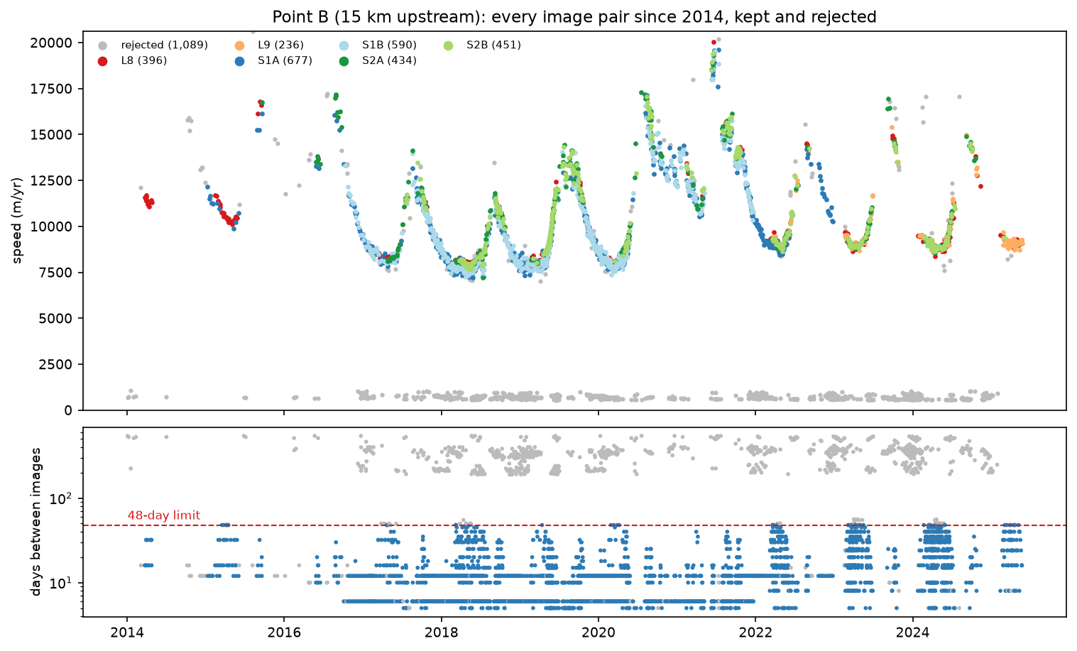

The figure shows why filtering on date_dt matters so much on fast glaciers. Over 200 days, ice moving at 10 km/yr travels more than 5 km. The surface changes beyond recognition and the offset exceeds the search window, so the correlation peak comes from something else and the result is far too slow. A median over all pairs would be badly biased. On slow ice the trade-off reverses: at point D (438 m/yr) the relative-error test removed most pairs, because a v_error of a few tens of m/yr is more than 15% of the speed. For slow ice, use an absolute error limit instead.

Step 5: seasonal cycle and multi-year change

With clean pairs, compute monthly medians at each point. For the seasonal cycle, express each month relative to a centred 12-month mean, so that the multi-year trend drops out, then take the median for each calendar month.

for k, f in filt.items():
    g = f[f.keep]
    m = g.v.resample("MS").median()
    trend = m.rolling(13, center=True, min_periods=7).mean()
    rel = (100 * (m / trend - 1)).groupby(m.index.month).median()

       km  pairs  peak month  min month  seasonal range %  2014 median  2017 median  2024 median
point
A       5   1267           9          3              54.6          NaN      10025.0       9457.0
B      15   2784           8          4              49.1      11400.0       9114.0       9001.0
C      30   4083          10          5              13.8       4574.0       4000.0       3976.0
D      60   1742           6         11              12.8        444.5        475.0        445.0

ITS_LIVE climatological seasonal fit (2014-2024) at the points:
  A: v0 11,810 m/yr, amplitude 2,104 m/yr (18%), peak on day 259 (~16 Sep)
  B: v0 10,223 m/yr, amplitude 2,698 m/yr (26%), peak on day 249 (~06 Sep)
  C: v0 3,829 m/yr, amplitude 239 m/yr (6%), peak on day 267 (~24 Sep)
  D: v0 438 m/yr, amplitude 2 m/yr (0%), peak on day 172 (~21 Jun)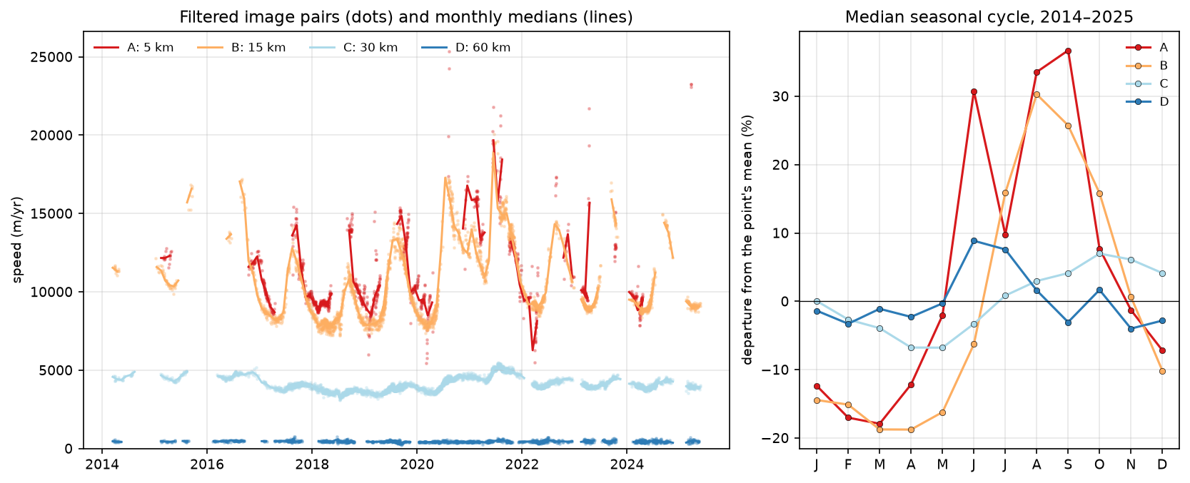

The lower trunk is fastest in late summer and slowest in spring, a range of 55% at point A and 49% at point B. ITS_LIVE’s own sine-wave fit agrees on the timing (peaks on about 16 and 6 September) but gives a smaller amplitude, 18–26% of the mean. That is expected: Jakobshavn’s cycle is not a sine wave. It speeds up sharply in early summer, when the front retreats and the mélange that buttresses it breaks up, and slows gradually through the winter as the front advances again. Upstream, the cycle is much weaker: 6% in the ITS_LIVE fit at point C, and nothing measurable at point D.

Step 6: strain rates and flow direction

Spatial derivatives of the velocity field give the strain rate: how fast the ice stretches or compresses. Derivatives amplify noise, so smooth the climatological components first. We use a Gaussian with σ = 5 pixels (600 m), a few times the ice thickness. The longitudinal strain rate is the stretching rate along the flow direction. The effective strain rate is the second invariant of the strain-rate tensor, with the vertical component taken from incompressibility. It is the quantity that enters Glen’s flow law for ice.

dx, dy = float(x[1] - x[0]), float(y[1] - y[0])            # dy is negative: y decreases down the rows
w = ndimage.gaussian_filter(np.isfinite(vx0.values).astype(float), 5)
u = ndimage.gaussian_filter(np.nan_to_num(vx0.values), 5) / np.maximum(w, 1e-6)
v = ndimage.gaussian_filter(np.nan_to_num(vy0.values), 5) / np.maximum(w, 1e-6)
mask = (w > 0.9) & (landice.values == 1)
dudy, dudx = np.gradient(u, dy, dx)
dvdy, dvdx = np.gradient(v, dy, dx)
exy = 0.5 * (dudy + dvdx)
speed = np.hypot(u, v)
e_long = (u ** 2 * dudx + u * v * (dudy + dvdx) + v ** 2 * dvdy) / speed ** 2     # along-flow strain rate, 1/yr
e_eff = np.sqrt(0.5 * (dudx ** 2 + dvdy ** 2 + (dudx + dvdy) ** 2) + exy ** 2)     # effective strain rate, 1/yr

point A: longitudinal strain rate +0.015 /yr, effective 0.394 /yr
point B: longitudinal strain rate +0.720 /yr, effective 0.871 /yr
point C: longitudinal strain rate +0.291 /yr, effective 0.950 /yr
point D: longitudinal strain rate +0.009 /yr, effective 0.015 /yr
max longitudinal stretching on the flowline: 1.12 /yr at 12.4 km
max compression on the flowline: -1.09 /yr at 0.0 km

For flow direction, plot unit vectors with quiver, so that arrow length does not swamp the slow ice:

st = 25                                                  # one arrow every 25 pixels = 3 km
X, Y = np.meshgrid(x[::st], y[::st])
U, V = u[::st, ::st], v[::st, ::st]
S = np.hypot(U, V)
q = (S > 100) & mask[::st, ::st]
axs[1].quiver(X[q], Y[q], (U / S)[q], (V / S)[q], color="white", scale=32, width=0.003, headwidth=4)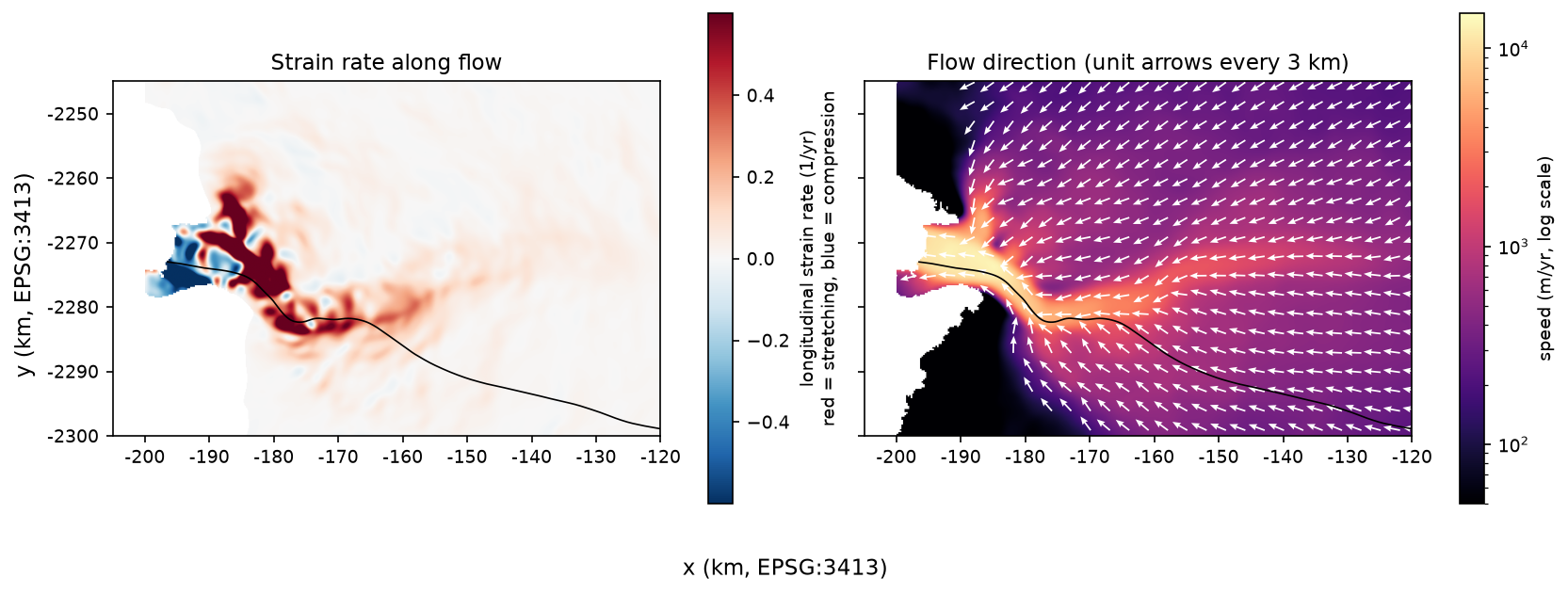

Ice entering the trunk at point B is stretched at 0.72 per year: a 100 m length of ice grows by about 20 cm every day. The maximum, 1.12 per year, is 12.4 km above the ice edge, where the trunk is accelerating hardest. Rates like these open the dense crevasse fields that make the lower glacier impassable. Close to the ice edge the flow is compressive (−1.09 per year), because the front is buttressed by the mélange and the fjord walls. Point C has modest stretching along the flow (0.29 per year) but a high effective strain rate (0.95 per year), so other components, mainly shear, dominate there.

Step 7: save the results

out = pd.DataFrame({"dist_km": dist_km, "x": line[:, 0], "y": line[:, 1], "v0": spd(line[:, ::-1]), "e_long": along})
out = out.join(pd.DataFrame(prof.values.T, columns=[f"v_{y_}" for y_ in years]))
out.to_csv(OUT / "flowline_profiles.csv", index=False, float_format="%.3f")
pd.concat({k: f[f.keep][["v", "v_error", "date_dt", "sensor"]] for k, f in filt.items()}, names=["point"]).to_csv(
    OUT / "point_timeseries_filtered.csv", float_format="%.2f")

flowline_profiles.csv has one row per flowline vertex, with its distance, coordinates in EPSG:3413, climatological speed, strain rate and the annual speed for every year from 1984 to 2025. point_timeseries_filtered.csv has every kept image pair at points A–D. To use the flowline in QGIS, write x and y as points with geopandas in EPSG:3413.

Pitfalls and limitations

• ITS_LIVE measures surface velocity. It says nothing directly about the bed or the ice flux. To get discharge you need ice thickness, for example from BedMachine Greenland.
• Failed matches on fast ice. Long image pairs, pairs across the melt season, and pairs over fresh snow can report speeds that are far too low. Filter by date_dt and look at the scatter before you trust a mean.
• Relative error filters penalise slow ice. At point D only 24% of pairs survived the 15% test. Use an absolute error limit for slow-moving ice, or the v_error weighting used in the composites.
• Uneven sampling. Sentinel-1B failed in December 2021, and optical sensors see nothing in the polar night. Monthly medians, averaged month by month, give fairer annual figures than the median of all pairs.
• Partial years and a moving front. The 2025 composite was built from data up to May 2025 only. The ice edge also moves by kilometres each season, so a pixel near the front may be glacier in one image and mélange or open water in the next. We stopped the flowline at the static land-ice mask for that reason.
• Smoothing controls strain rates. Peak strain rates depend strongly on the smoothing length: less smoothing gives higher, noisier peaks. Report the smoothing with any strain-rate figure.
• Datacube versions. ITS_LIVE reprocesses and updates its cubes. The catalogue pointed to v2-updated-october2024 cubes with data up to May 2025. Re-running later may return more pairs and slightly different numbers.

Frequently asked questions

How do I get glacier velocity data in Python?

Use NASA ITS_LIVE. Download the public catalogue (catalog_v02.json), find the datacube whose footprint contains your glacier, and open its zarr_url with xr.open_dataset(url, engine="zarr"). No account is needed. For maps, open the matching annual composite (composite_zarr_url). The itslive Python package wraps the same steps if you prefer a higher-level interface.

What is the difference between the ITS_LIVE datacube and the composites?

The datacube holds every individual image-pair velocity field: tens of thousands of layers, each an average over its own time separation, chunked for fast time series at a point. The annual composites are one error-weighted mosaic per year, plus a fitted 2014–2024 climatology with a seasonal amplitude and phase. Use composites for maps and profiles, and the datacube for seasonal and short-term change.

How does feature tracking measure glacier velocity?

It matches small image chips between two images of the same place taken days to months apart. The best match, found by normalised cross-correlation and refined to sub-pixel precision, gives the displacement. Divided by the time between the images, that is the velocity. ITS_LIVE uses the autoRIFT algorithm on Landsat, Sentinel-2 and Sentinel-1 pairs.

Why do some ITS_LIVE velocities look far too slow?

Usually because matching failed. On fast glaciers, image pairs that are hundreds of days apart see the surface change beyond recognition, so the correlation locks onto something else. At Jakobshavn such pairs report about 700 m/yr where the ice moves at about 10,000 m/yr. Filter by time separation (date_dt), error (v_error) and a rolling-median test.

How fast does Jakobshavn Isbræ flow?

In the 2014–2024 ITS_LIVE climatology, the fastest ice in the cube moves at 15,195 m/yr, about 42 m per day. Annual speed 5 km above the ice edge rose from 6,208 m/yr in 1985 to 15,276 m/yr in 2007, fell to 9,569 m/yr in 2019 and was 10,489 m/yr in 2024. In summer, filtered image pairs 15 km upstream exceed 17,000 m/yr.

Can I use ITS_LIVE for mountain glaciers such as the Aletsch?

Yes. The datacubes cover glaciers worldwide, in UTM projections outside the polar regions, and the same code works if you change LON and LAT. Mountain glaciers are slower and narrower than Jakobshavn, so use an absolute error threshold, check that the 120 m grid resolves the glacier, and expect more gaps in winter from snow and shadow.

Next steps

• Map snow, the other half of the cryosphere, in snow cover mapping with NDSI in Python.
• Measure millimetre-scale ground movement with radar interferometry in InSAR ground deformation in Python. Feature tracking is the large-displacement counterpart of InSAR.
• Compute slope and aspect of the ice surface from a DEM with raster terrain analysis with rasterio.
• Build gridded time series from STAC instead of Zarr with NDVI time series in Python with Sentinel-2 and odc-stac.
• Watch the calving front itself: the water-edge methods in coastal erosion and shoreline change from Sentinel-2 and Sentinel-1 SAR flood mapping work on the fjord too.
• Put the flowline on an interactive map with Folium, or browse more open data in the TechnicalGIS data catalogue.

Data and licences

• Glacier velocities: velocity data generated using auto-RIFT (Gardner et al., 2018; Lei et al., 2021) and provided by the NASA MEaSUREs ITS_LIVE project (Gardner et al., doi:10.5067/JQ6337239C96). ITS_LIVE image-pair datacube ITS_LIVE_vel_EPSG3413_G0120_X-150000_Y-2250000.zarr (v2, updated October 2024, data to 28 May 2025) and annual composite ITS_LIVE_velocity_EPSG3413_120m_X-150000_Y-2250000.zarr (v2, updated September 2025), read from the public its-live-data AWS S3 bucket on 21 October 2026. ITS_LIVE data are openly available with no restrictions on use; the attribution follows the project’s recommended wording at its-live.jpl.nasa.gov.
• Underlying imagery: Landsat courtesy of the U.S. Geological Survey; contains modified Copernicus Sentinel-1 and Sentinel-2 data, processed by ITS_LIVE.
• Country outlines: Natural Earth, public domain.
• References: Gardner, A. et al., MEaSUREs ITS_LIVE Regional Glacier and Ice Sheet Surface Velocities, Version 2 (NSIDC-0776), NASA National Snow and Ice Data Center DAAC, doi:10.5067/JQ6337239C96; Gardner, A. S. et al. (2018), “Increased West Antarctic and unchanged East Antarctic ice discharge over the last 7 years”, The Cryosphere 12(2), 521–547, doi:10.5194/tc-12-521-2018; Lei, Y., Gardner, A. and Agram, P. (2021), “Autonomous Repeat Image Feature Tracking (autoRIFT) and its application for tracking ice displacement”, Remote Sensing 13(4), 749; Joughin, I., Abdalati, W. and Fahnestock, M. (2004), “Large fluctuations in speed on Greenland’s Jakobshavn Isbræ glacier”, Nature 432, 608–610; Khazendar, A. et al. (2019), “Interruption of two decades of Jakobshavn Isbrae acceleration and thinning as regional ocean cools”, Nature Geoscience 12, 277–283.
• Code: glacier_velocity_its_live.py, tested with Python 3.12.0, xarray 2026.9.0, zarr 3.4.1, dask 2026.8.0, numpy 2.5.4, pandas 3.0.6, scipy 1.18.1, geopandas 1.2.0 and matplotlib 3.11.2.