Coastal erosion and shoreline change from Sentinel-2 in Python (Holderness, 2017–2026)
Measure shoreline change on one of Europe's fastest-eroding coasts with free Sentinel-2 imagery and Python: MNDWI and Otsu thresholding, sub-pixel shorelines with find_contours, shore-normal transects, a tide correction from open tide-gauge data, end-point and linear regression rates, and an honest comparison with East Riding of Yorkshire Council's cliff monitoring.
- Level
- Advanced
- Tested with
- Python 3.12
- Source code
- Download scripts
Key takeaways
- A shoreline from Sentinel-2 is the MNDWI land–water boundary: threshold MNDWI with Otsu's method, then trace it at sub-pixel precision with skimage.measure.find_contours.
- Of 751 scenes of the Holderness coast from 2017 to 2026, 551 gave a shoreline and 545 crossed the transects, giving 69,486 shoreline positions on 332 transects 100 m apart.
- The tide matters more than the erosion. On a beach sloping about 1:27, the waterline moves 27 m for every metre of tide, so correcting with a tide model fitted to open Environment Agency gauge data halved the scatter from 41.6 m to 21.1 m and the rate uncertainty from ±2.01 to ±1.01 m/yr.
- The tide-corrected waterline retreated at a median of 1.01 m/yr from 2017 to 2026 (uncorrected: 0.72 m/yr). Where it lines up with the council's 62 cliff-monitoring profiles, the median is 1.08 m/yr, against 1.87 m/yr for the cliff top from 1989 to 2026.
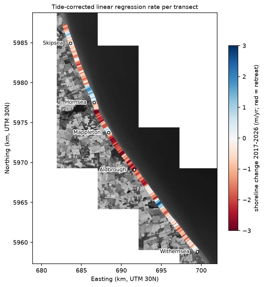
- The satellite and the council agree on the pattern (Spearman ρ = 0.60): sediment builds up north of the Hornsea and Mappleton defences, and erosion jumps just south of them.
Before you start
- Comfortable with NumPy, pandas, shapely and rasterio (the Sentinel-2 Lake Mead tutorial introduces STAC searches and Cloud Optimised GeoTIFFs)
- Python 3.10+ with pystac-client, planetary-computer, rasterio, numpy, scipy, pandas, geopandas, shapely, pyproj, scikit-image, utide, pypdf, requests and matplotlib
- An internet connection: imagery is streamed from the Microsoft Planetary Computer and tide data come from the Environment Agency, and neither needs an account or API key
Short answer: to measure coastal erosion from satellite imagery in Python, take every Sentinel-2 image of the coast and, for each one: compute MNDWI = (B03 − B11) / (B03 + B11), choose a land–water threshold with Otsu’s method, and trace the shoreline at sub-pixel precision with skimage.measure.find_contours. Then cast shore-normal transects along the coast, record where each shoreline crosses each transect, correct each position for the tide at the time of the image, and fit a line through the positions over time. The slope is the linear regression rate (LRR) in metres per year. This is the method behind the open-source CoastSat toolkit, written here from scratch so that every step is visible.
The Holderness coast in East Yorkshire is one of the fastest-eroding coastlines in Europe. Its cliffs are soft glacial till, and East Riding of Yorkshire Council, which monitors them twice a year, describes average losses of up to about 4.5 m per year at the worst sites. Whole villages, such as Owthorne near Withernsea, have been lost to the sea. That makes it a good, demanding test: the change is real and well documented, but the beach in front of the cliffs is wide and gently sloping, so the tide moves the waterline far more than a year of erosion does. In this tutorial we map 33 km of coast from Skipsea to Withernsea with every Sentinel-2 image from January 2017 to October 2026, and compare the result with the council’s measurements.
You will learn how to:
- read the council’s cliff-monitoring profiles from its published PDF;
- build a harmonic tide model from open Environment Agency tide-gauge data with
utide, and check it on held-out days; - search and stream ten years of Sentinel-2 L2A from the Microsoft Planetary Computer, reading only the pixels along the coast;
- extract a sub-pixel shoreline from each image with MNDWI, Otsu and
find_contours; - cast shore-normal transects and intersect them with every shoreline;
- estimate the beach slope from the data, correct for the tide and compute EPR and LRR with confidence intervals;
- compare the rates with the East Riding cliff-top rates, and explain why they differ.
All outputs below are real results from coastal_erosion_shorelines.py, run on 19 October 2026 with Python 3.12, pystac-client 0.9.0, rasterio 1.5.2, scikit-image 0.26.0 and utide 0.4.0.
How satellite shoreline mapping works
A satellite cannot see the cliff top or the legal mean high water line. It sees the waterline: the boundary between wet and dry at the moment the image was taken. Three things move that boundary:
- Erosion or accretion of the beach, which is the signal we want;
- The tide: on a beach with a slope of 1:30, a 2 m rise in water level moves the waterline 60 m inland;
- Waves and wave run-up, plus short-lived changes in the beach such as storm cut-back and migrating sandbanks.
Sentinel-2 has 10 m pixels in the visible bands and a revisit of 2–5 days. One image is too uncertain to measure 1–2 m of annual retreat, but hundreds of images, each with a tide correction, pin the trend down to about ±1 m/yr. This is the principle of CoastSat (Vos et al., 2019), the most widely used open-source toolkit for satellite-derived shorelines. CoastSat classifies pixels with a small neural network, refines the threshold at the sand–water boundary, corrects for the tide with a global tide model and measures change along transects. Here we use a simpler MNDWI and Otsu classifier, a tide model fitted to local gauges, and a beach slope estimated from the shorelines themselves.
Step 1: the council’s cliff-monitoring profiles
East Riding of Yorkshire Council surveys the cliff top along fixed profiles every spring and autumn, and publishes a table of losses and long-term rates as a PDF. Each row has the profile’s two end points in British National Grid. We parse it with pypdf and a regular expression:
ERYC_URL = "https://www.eastriding.gov.uk/download/east-riding-coastal-erosion-statistics/"pdf_path = DATA / "eryc_cliff_erosion_table.pdf"if not pdf_path.exists(): r = get(ERYC_URL, headers={"User-Agent": "Mozilla/5.0 (TechnicalGIS tutorial script)"}) # blocks default agents r.raise_for_status() pdf_path.write_bytes(r.content)text = "\n".join(p.extract_text() for p in PdfReader(pdf_path).pages)NUM = r"(\d{6,7}\.\d)"rows = []for line in text.splitlines(): m = re.match(rf"^(\d+)\s+(.+?)\s+{NUM}\s+{NUM}\s+{NUM}\s+{NUM}\s+(.*)$", line.strip()) if not m: continue vals = re.findall(r"-?\d+\.\d+", m.group(7).replace("*", "")) rows.append({"profile": int(m.group(1)), "location": m.group(2), "e1": float(m.group(3)), "n1": float(m.group(4)), "e2": float(m.group(5)), "n2": float(m.group(6)), "defended": "Defended" in m.group(7), # columns: loss Mar-Sep 2025, loss Sep 2025-Mar 2026, rate 1852-1989, rate 1989-2026, height, max loss "rate_1989_2026": float(vals[3]) if len(vals) >= 6 else np.nan, "loss_last_year": float(vals[0]) + float(vals[1]) if len(vals) >= 6 else np.nan})eryc = pd.DataFrame(rows)eryc["length_m"] = np.hypot(eryc.e2 - eryc.e1, eryc.n2 - eryc.n1)bad = eryc[eryc.length_m > 3000]eryc = eryc[eryc.length_m <= 3000].copy()Two profiles have a coordinate with a missing digit (their “lines” would be tens of kilometres long), so we drop them. We keep profiles 22 to 89, from the North Caravan Park at Skipsea to the north end of the Withernsea sea wall:
=== East Riding erosion profiles (PDF table) ===108 profiles parsed; dropped 2 with a typing error in the coordinates: [10, 71]study stretch: profiles 22-89, 64 profiles, 64 with a 1989-2026 ratecouncil cliff-top erosion rate 1989-2026: median 1.85 m/yr, range 0.07-3.28 m/yr profile location rate_1989_2026 loss_last_year 22 North Boundary of North Caravan Park, Skipsea 1.50 1.60 23 South end of Seaside Caravan Park, Ulrome 1.11 0.77 24 Between defences opposite Southfield Lane, Ulrome 1.09 1.02 25 North end of Green Lane, Skipsea 1.22 0.45 26 South of Green Lane, Skipsea 0.95 0.00 27 Opposite Skipsea village 1.12 0.90 28 Opposite bungalows to south of Skipsea 1.30 0.95 29 To south of Withow Gap, Skipsea 1.40 0.00The council’s long-term median for this stretch is 1.85 m/yr, ranging from 0.07 m/yr just north of Hornsea’s sea wall to 3.28 m/yr just south of Mappleton. Note the last column: in the latest year, some profiles lost nothing and others lost 1.6 m. Cliff retreat on Holderness is episodic, so short records are noisy, whichever way they are measured.
Step 2: a tide model from open tide-gauge data
Every Sentinel-2 image of Holderness is taken at about 11:10 UTC, at whatever state of the tide that happens to be. To correct for it we need the tide height at each overpass, from 2017 onwards.
The obvious sources each have a catch. Global ocean tide models such as FES2014 and FES2022, which CoastSat uses through pyfes, need a free AVISO account to download. The National Tidal and Sea Level Facility (NTSLF) runs the UK’s A-class tide gauges and publishes predictions, but its nearest gauges are Whitby and Immingham, neither on this coast, and its quality-controlled historical data come through the British Oceanographic Data Centre, which needs registration. So we use the Environment Agency’s open real-time gauges at Bridlington (north of the study area) and Spurn Point (south of it). They report every 15 minutes, need no key and are licensed under the Open Government Licence. The API serves the last few weeks, and a daily archive file goes back about a year. We take one archive day per month plus the recent weeks, and fit a harmonic tide model with utide, which we can then run at any time in the past:
GAUGES = {"Bridlington": ("L3001-level-tidal_level-i-15_min-m", 54.0798), "Spurn Point": ("L3370-level-tidal_level-i-15_min-mAOD", 53.5779)}...# Bridlington harbour dries out near low water: the gauge then sits flat at its floor (-1.61 m).# Those readings are not the tide, so drop everything within 3 cm of each gauge's minimum.floor = tides.groupby("gauge")["level"].transform("min")dry = (tides.gauge == "Bridlington") & (tides.level <= floor + 0.03)tides = tides[~dry]...CONSTITUENTS = ["M2", "S2", "N2", "K2", "K1", "O1", "P1", "Q1", "M4", "MS4", "MN4", "M6", "2N2", "MU2", "NU2", "L2"]HOLDOUT = ["2026-01-01", "2026-04-01", "2026-07-01"]models, val = {}, []for name, (_, lat) in GAUGES.items(): g = tides[tides.gauge == name] fit = g[~g.day.isin(HOLDOUT)] coef = utide.solve(fit.time.dt.tz_localize(None).values, fit.level.values - fit.level.mean(), lat=lat, constit=CONSTITUENTS, method="ols", conf_int="none", trend=False, verbose=False) coef["offset"] = fit.level.mean() models[name] = coef=== tide gauge readings (Environment Agency, 15-minute) === readings first last daysgaugeBridlington 3552 2025-11-01 00:00:00+00:00 2026-10-19 15:15:00+00:00 41Spurn Point 3897 2025-11-01 00:00:00+00:00 2026-10-19 15:15:00+00:00 41dropped 345 Bridlington readings sitting on the dry-harbour floor (-1.61 m)
=== harmonic tide model (utide) ===Bridlington 16 constituents; largest amplitudes (m): M2 1.82, S2 0.63, N2 0.33, K2 0.19, O1 0.18Spurn Point 16 constituents; largest amplitudes (m): M2 2.09, S2 0.73, N2 0.38, O1 0.20, K2 0.19hold-out days, predicted minus observed (m): rmse biasgauge Bridlington Spurn Point Bridlington Spurn Pointday2026-01-01 0.58 0.65 -0.54 -0.572026-04-01 0.22 0.23 0.18 0.182026-07-01 0.15 0.15 0.09 0.08The main lunar tide, M2, has an amplitude of 1.8–2.1 m, so the spring range on this coast is about 5 m. On two of the held-out days the model is within 0.15–0.23 m. On 1 January 2026 it is about 0.55 m too low at both gauges at once: a storm surge, which no astronomical tide model can predict. For each transect, the script interpolates the two gauges’ predictions by latitude.
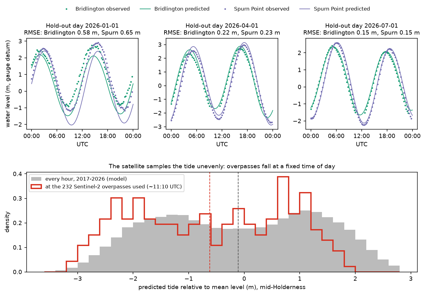
The bottom panel shows why the correction matters. A sun-synchronous satellite passes at the same local time every day, and spring tides recur at roughly the same times of day at any one place, so the satellite always sees spring tides at a similar stage. At about 11:10 UTC on Holderness that stage is nearer low water than high water. The images are therefore biased towards low water, and the mix of tides changes from year to year with the 18.6-year lunar nodal cycle and with which scenes happen to be cloud-free.
Step 3: search ten years of Sentinel-2
The coast lies in Sentinel-2 tile 30UXE, seen from two relative orbits. We search the Planetary Computer’s STAC API for every L2A scene of that tile with less than 80% cloud. Some dates were reprocessed and appear twice, so we keep the newer processing baseline:
catalog = pystac_client.Client.open(STAC_URL)items = list(catalog.search(collections=["sentinel-2-l2a"], bbox=bbox_ll, datetime=PERIOD, query={"s2:mgrs_tile": {"eq": TILE}, "eo:cloud_cover": {"lt": 80}}).items())best = {}for it in items: # a few dates exist twice (original and reprocessed): keep the newest processing baseline key = (it.datetime.date(), it.properties["sat:relative_orbit"]) if key not in best or it.properties["s2:processing_baseline"] > best[key].properties["s2:processing_baseline"]: best[key] = ititems = sorted(best.values(), key=lambda i: i.datetime)=== Sentinel-2 search ===751 scenes of tile 30UXE with tile cloud cover < 80%, 2017-01-02 to 2026-10-17137 38437 367Step 4: read only the pixels along the coast
A full Sentinel-2 tile is 10,980 × 10,980 pixels, and we need about 1 km either side of a 33 km coastline. Cloud Optimised GeoTIFFs are stored in 512 × 512 pixel blocks, so the script lists the blocks that the corridor around the council profiles touches (14 of the 484) and reads just those, from 751 scenes. The 20 m SWIR band B11 is resampled to 10 m with bilinear interpolation; the scene classification layer (SCL) is read first, and a scene is abandoned before the 10 m bands are downloaded if cloud covers too much of the coast:
def reflectance(item, dn: np.ndarray) -> np.ndarray:    """Surface reflectance; baseline 04.00+ (from January 2022) adds 1000 to every digital number."""    offset = 1000 if float(item.properties["s2:processing_baseline"]) >= 4.0 else 0    return np.where(dn > 0, (dn.astype("float32") - offset) / 10000, np.nan)

BAD_SCL = [0, 1, 3, 8, 9, 10]           # no data, defective, cloud shadow, cloud medium/high, cirrus

def scene_mndwi(item, zone=None, min_clear=0.0): """MNDWI = (green - SWIR1) / (green + SWIR1) and a validity mask (clear, observed pixels). Reads the small SCL band first and gives up early if too little of `zone` is clear.""" item = planetary_computer.sign(item) scl = read_band(item, "SCL", 2) bad = ndimage.binary_dilation(np.isin(scl, BAD_SCL) & in_corridor, iterations=3) | (scl == 0) if zone is not None and (~bad[zone]).mean() < min_clear: return None, None green = reflectance(item, read_band(item, "B03", 1)) swir = reflectance(item, read_band(item, "B11", 2, Resampling.bilinear)) with np.errstate(divide="ignore", invalid="ignore"): mndwi = (green - swir) / (green + swir) valid = ~bad & np.isfinite(mndwi) & in_corridor return mndwi, valid=== analysis mosaic ===14 blocks of 512 x 512 pixels at 10 m; mosaic 2048 x 3584 pixels (20.5 x 35.8 km), EPSG:32630We use MNDWI rather than NDWI (green and near-infrared) because shortwave infrared is absorbed almost completely by even a thin film of water, while wet sand still reflects strongly in the near-infrared. MNDWI therefore separates sea from wet beach more cleanly, and is less affected by suspended sediment, which is abundant off Holderness because the eroding till releases huge volumes of mud.
Step 5: a reference shoreline and shore-normal transects
Transects need a baseline. We take the median MNDWI of the 20 least cloudy scenes, threshold it with Otsu, trace the longest contour, trim it to the council’s first and last profiles, and smooth it with a 510 m running mean so that the transects are perpendicular to the overall trend of the coast, not to every small wiggle in the waterline:
ref_mndwi = np.load(ref_path)ref_thr = threshold_otsu(ref_mndwi[np.isfinite(ref_mndwi)])contours = find_contours(np.nan_to_num(ref_mndwi, nan=-1), ref_thr, mask=np.isfinite(ref_mndwi))longest = max(contours, key=len)ref_line = LineString(np.column_stack(rc_to_xy(longest[:, 0], longest[:, 1])))...smooth = np.column_stack([ndimage.uniform_filter1d(pts[:, k], 51, mode="nearest") for k in (0, 1)])ref_smooth = LineString(smooth)Then every 100 m along the baseline, a transect runs 250 m landward and 350 m seaward along the local normal:
SPACING, LAND, SEA = 100, 250, 350transects = []for s in np.arange(50, ref_smooth.length - 50, SPACING): p0, p1 = np.array(ref_smooth.interpolate(s - 25).coords[0]), np.array(ref_smooth.interpolate(s + 25).coords[0]) t = (p1 - p0) / np.linalg.norm(p1 - p0) n = np.array([t[1], -t[0]]) # right-hand normal; the sea is to the east if n[0] < 0: n = -n c = np.array(ref_smooth.interpolate(s).coords[0]) transects.append({"chainage_km": s / 1000, "geometry": LineString([c - LAND * n, c + SEA * n]), "x0": c[0] - LAND * n[0], "y0": c[1] - LAND * n[1], "nx": n[0], "ny": n[1]})tr = gpd.GeoDataFrame(transects, crs=CRS)=== reference shoreline ===median MNDWI of the 20 least cloudy scenes; Otsu threshold 0.163reference shoreline 33.3 km long, Skipsea to Withernsea332 transects, 100 m apart, 250 m landward and 350 m seaward of the reference line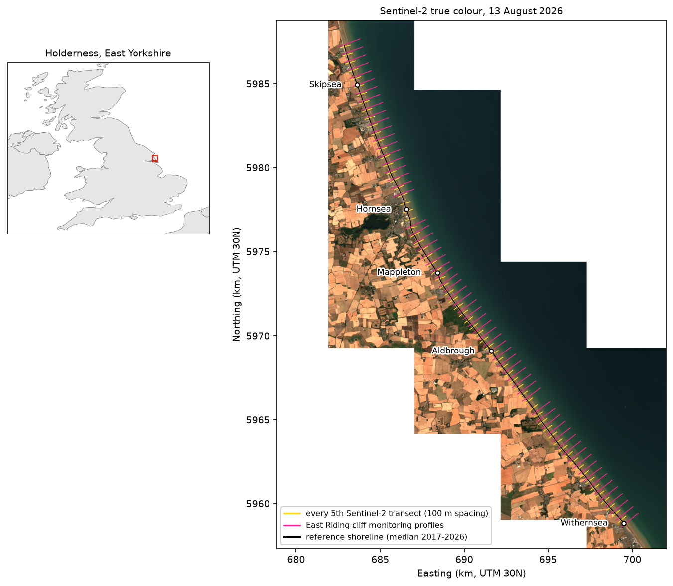
Step 6: extract a sub-pixel shoreline from every scene
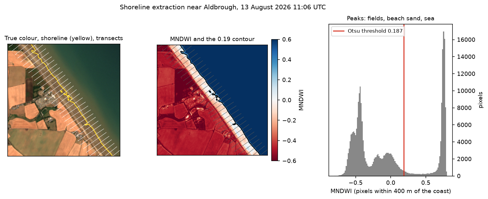
For each scene, the script keeps the clear pixels within 400 m of the baseline, chooses an Otsu threshold from just those pixels, and traces the threshold contour with find_contours. Restricting Otsu to the shore zone matters: over the whole image, the histogram is dominated by fields and open sea, and the threshold would ignore the beach. Scenes in which less than 20% of the shore zone is clear are skipped after reading only the SCL band. Each result is cached, so later runs are fast:
def extract_shoreline(item):    """Otsu threshold on MNDWI in the shore zone, then the sub-pixel 'marching squares' contour."""    path = CACHE / "shorelines" / f"{item.id}.npz"    if path.exists():        return dict(np.load(path))    mndwi, valid = scene_mndwi(item, zone, MIN_CLEAR)    if mndwi is None:        res = {"status": np.array("cloudy")}    else:        ok = valid & zone        thr = threshold_otsu(mndwi[ok])        cs = find_contours(np.where(ok, mndwi, -1).astype("float32"), thr, mask=ok)        cs = [np.column_stack(rc_to_xy(c[:, 0], c[:, 1])) for c in cs if len(c) >= 10]        coords = np.concatenate([np.vstack([c, [np.nan, np.nan]]) for c in cs]) if cs else np.empty((0, 2))        clear_tr = np.array([ok.ravel()[s].mean() for s in samples])        res = {"status": np.array("ok"), "threshold": np.array(thr), "zone_clear": np.array(ok[zone].mean()),               "contours": coords, "transect_clear": clear_tr}    np.savez_compressed(path, **res)    return res

with ThreadPoolExecutor(6) as ex: results = list(ex.map(extract_shoreline, items))=== shoreline extraction ===751 scenes processed in 1 s: 551 with a shoreline, 200 with less than 20% of the shore zone clearOtsu MNDWI thresholds: median 0.174, 5th-95th percentile 0.052 to 0.275The “1 s” is from the cached rerun that produced this output; the first run took about 4.5 minutes on a fast connection. The thresholds vary from 0.05 to 0.28 between scenes, which is why a fixed MNDWI threshold of 0 is a poor choice here.
Step 7: intersect every shoreline with every transect
Each shoreline is intersected with each transect that is at least 90% cloud-free in that scene. If a transect crosses the contour several times more than 50 m apart (usually breaking waves, a pool on the beach or a cloud edge), that crossing is rejected; otherwise the median is used. The position x is measured from the reference line, positive seaward. Each observation also gets the predicted tide at its overpass time:
for item, r in zip(items, results): if str(r["status"]) != "ok" or len(r["contours"]) == 0: continue c = r["contours"] parts = np.split(c, np.where(np.isnan(c[:, 0]))[0]) lines = MultiLineString([p[~np.isnan(p[:, 0])] for p in parts if (~np.isnan(p[:, 0])).sum() >= 2]) for j, g in enumerate(tr_geoms): if r["transect_clear"][j] < MIN_TR_CLEAR: continue hit = g.intersection(lines) if hit.is_empty: continue d = np.array([g.project(p) for p in getattr(hit, "geoms", [hit])]) - LAND if d.max() - d.min() > MAX_SPREAD: # several crossings far apart: whitewater, ords, cloud edge continue records.append((item.id, item.datetime, j, float(np.median(d))))=== shoreline positions on transects ===69,486 shoreline positions from 545 scenes (2017-01-02 to 2026-10-17)positions per transect: median 208, min 156overpass time 11:06 to 11:25 UTC; predicted tide at overpass -3.29 to +1.99 m (median -0.58 m)Step 8: tide correction and change rates
How far does the waterline move per metre of tide? That is the inverse of the beach slope, and it varies along the coast. Rather than assume a slope, we estimate it from the data. For each transect we fit
x = a + r · t + k · tide
where r is the trend and k is the waterline shift per metre of tide (negative, because a higher tide pushes the waterline landward). Two passes of least squares remove outliers beyond three robust standard deviations. k is noisy from transect to transect, so it is smoothed alongshore with an 11-transect running median. Each position is then moved to mean sea level, and the LRR, its 95% confidence interval and the EPR are computed:
for j, g in obs.groupby("transect"):    X = np.column_stack([np.ones(len(g)), g.year - 2017, g.tide])    beta, keep = robust_fit(X, g.x.values)    obs.loc[g.index, "keep"] = keep    rows.append({"transect": j, "k_raw": beta[2], "n": keep.sum()})fit = pd.DataFrame(rows).set_index("transect")# The tide coefficient k (metres of shoreline shift per metre of tide) is -1 / beach slope. It is noisy# transect by transect, so smooth it alongshore with an 11-transect (1.1 km) running median.fit["k"] = fit.k_raw.rolling(11, center=True, min_periods=1).median().clip(upper=-1)fit["beach_slope"] = -1 / fit.kobs = obs.join(fit.k, on="transect")obs["x_corr"] = obs.x - obs.k * obs.tide          # shoreline position at mean sea level
out = []t0, t1 = obs.time.min(), obs.time.max()for j, g in obs[obs.keep].groupby("transect"): lrr, ci = ols_rate(g.year, g.x_corr) lrr_raw, ci_raw = ols_rate(g.year, g.x) first = g[g.time < t0 + pd.Timedelta(days=365)] last = g[g.time > t1 - pd.Timedelta(days=365)] epr = (last.x_corr.median() - first.x_corr.median()) / ((last.year.median() - first.year.median()))=== tide correction ===tide coefficient k (m of shoreline shift per m of tide): median -27.2, equivalent beach slope 1:27 (5th-95th pct 1:17 to 1:36)scatter about the trend: median 41.6 m without tide correction, 21.1 m with itoutliers removed: 2,423 of 69,486 positions (3.5%)
=== shoreline change rates (negative = landward retreat) ===LRR, tide-corrected: median -1.01 m/yr, IQR -1.75 to -0.23LRR, no tide correct: median -0.72 m/yrEPR (first vs last 12 months): median -0.32 m/yrmedian 95% CI half-width of LRR: 1.01 m/yr tide-corrected, 2.01 m/yr uncorrectedtransects with significant retreat (CI excludes 0): 164 of 332trend in predicted tide at overpass time: -0.4 cm/yr; times the median k that is a spurious +0.11 m/yr of apparent seaward shoreline motionThe fitted beach slope is about 1:27, between 1:17 and 1:36 along most of the coast. With a 5 m spring tidal range, that means the waterline sweeps across more than 100 m of beach twice a day. The tide correction halves the scatter (41.6 m to 21.1 m) and halves the uncertainty of the rate (±2.01 to ±1.01 m/yr).
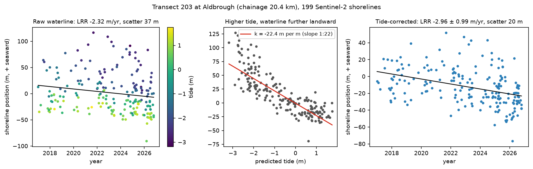
EPR or LRR? The end-point rate compares only the first and last 12 months, so it is at the mercy of the beach state in those two years. Here its median, −0.32 m/yr, is much smaller than the LRR. The LRR uses all 200 or so shorelines per transect and comes with a confidence interval, so it is the rate to report for satellite shorelines. Even so, only 164 of the 332 transects show retreat that is statistically distinguishable from zero over nine years.
Step 9: compare with East Riding of Yorkshire Council
For each council profile, the script finds where it crosses the reference line and averages the satellite rates of the transects within 150 m (three transects). Sixty-two profiles match: profiles 22 and 89, at the two ends, fall just outside the transects. The Hornsea sea front (profiles 42–44) is not in the council’s table.
=== comparison with East Riding of Yorkshire Council cliff-top rates ===62 council profiles matched to transectscouncil 1989-2026 cliff-top retreat: median 1.87 m/yrcouncil Mar 2025-Mar 2026 cliff loss: median 0.68 mSentinel-2 2017-2026 waterline retreat (tide-corrected LRR): median 1.08 m/yrSentinel-2 without tide correction: median 0.78 m/yrSpearman rank correlation, council rate vs Sentinel-2 retreat: 0.60 (p = 0.000)difference (Sentinel-2 minus council): median -0.81 m/yr, MAD 0.37 profiles council_1989_2026 s2_retreat s2_no_tidesectionSkipsea-Atwick (22-32) 10 1.17 0.71 1.52Atwick-Hornsea (33-46) 11 0.96 1.14 0.89Hornsea-Mappleton (47-59) 13 2.53 1.88 1.48Aldbrough (60-74) 14 2.18 1.41 0.40Aldbrough-Withernsea (75-89) 14 1.88 0.92 -0.48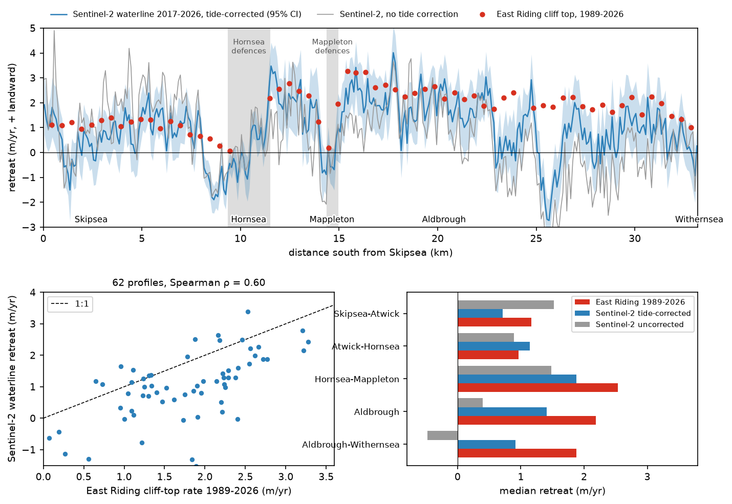
The pattern agrees well (Spearman ρ = 0.60):
- North of the Hornsea defences (8–10 km), the council’s cliff-top rates fall to 0.07–0.66 m/yr and the satellite waterline actually advanced. The sea walls and groynes hold sand moving south along the coast, so the beach builds up on their northern (updrift) side.
- Just south of Hornsea (11.5–13 km), the satellite rate jumps to a median of 2.2 m/yr and the council’s rates to 2.2–2.6 m/yr. This is the classic terminal groyne effect: the beach downdrift of the defences is starved of sand.
- The same happens at Mappleton, whose 1991 rock revetment and groynes hold the beach to the north (council: 0.19 m/yr at profile 51) while the cliffs to the south retreat at up to 3.28 m/yr. The fastest satellite retreat, 4.0 m/yr, is at 17.75 km near Cowden.
The level is lower. The satellite median is 1.08 m/yr where the council’s is 1.87 m/yr, and in the Tunstall area (profiles 77–83) the satellite shows 0 to 1.3 m/yr of retreat against the council’s 1.6–2.2 m/yr. Around Grimston (25–26 km), the waterline even advanced. Several real reasons explain this, and they are worth understanding before trusting any satellite erosion rate:
- Different features. The council measures the cliff top; Sentinel-2 measures the waterline on the beach in front of it. Over decades they retreat together, because the beach and the shore platform beneath it are cut back with the cliff. Over nine years, the beach can move independently by tens of metres.
- Different periods. 1989–2026 against 2017–2026. Holderness erosion is very episodic: in the council’s own latest year, the median loss was only 0.68 m, and 18 of the 62 profiles lost nothing at all. A 37-year average and a 9-year trend need not match.
- Ords. Holderness beaches have ords: low, sand-starved troughs, hundreds of metres long, that migrate slowly south along the coast. Where an ord sits, the beach is lower, the waterline is further landward and the cliff behind it erodes faster; when it moves on, the beach recovers. Depending on where the ords were at the start and end of the record, they add or remove metres of apparent change at individual transects, which is probably why the waterline advanced near Grimston.
- The tide model. The model is fitted to under a year of scattered gauge days, so its long-period constituents (including the 18.6-year nodal modulation) are not resolved. It also cannot predict surges of half a metre or more, and it is relative to each gauge’s mean level, not to Ordnance Datum. The gauges are also off the study coast: Spurn is at the mouth of the Humber, and Bridlington’s harbour dries at low water.
- Waves. Run-up and breaking waves move the visible waterline seaward or landward by up to tens of metres, depending on the conditions on the day. That is not corrected here.
So the honest summary is: Sentinel-2 reproduces where Holderness erodes fastest and where the defences change the pattern, and it confirms ongoing retreat of about 1 m/yr of the beach over 2017–2026, but it does not reproduce the council’s cliff-top rates one for one. For cliff-top rates, use the council’s surveys or lidar; satellite shorelines are best for long, continuous coverage of beaches, in places that are not surveyed.
Step 10: save the results
The script writes the rates per transect as CSV and GeoJSON (which opens directly in QGIS), the matched council profiles, and every shoreline position with its tide, so you can reanalyse them without downloading the imagery again:
rates.to_csv(OUT / "transect_rates.csv", float_format="%.3f")gpd.GeoDataFrame(rates, geometry=tr.geometry, crs=CRS).to_crs(4326).to_file(OUT / "transect_rates.geojson")cmp_.drop(columns=["e1_utm", "n1_utm", "e2_utm", "n2_utm"]).to_csv(OUT / "eryc_comparison.csv", index=False, float_format="%.3f")obs.to_csv(OUT / "shoreline_positions.csv", index=False, float_format="%.3f")Pitfalls and limitations
- Tide model. Under a year of gauge data is enough for the main constituents but not for long-period ones. With an AVISO account, FES2022 through
pyfesorpyTMDgives a global model with decades of validation; for UK work, the NTSLF and BODC records give longer gauge series. Whichever you use, check it against a gauge on held-out days, as in Step 2. - Storm surges. A 0.5 m surge on a 1:27 beach moves the waterline about 14 m. Use observed water levels instead of predictions where a gauge record covers the overpass time.
- Beach slope. The slope here is fitted from the shorelines, as CoastSat.slope does (Vos et al., 2020). It is reasonable on average, but it assumes a single slope over the whole intertidal zone and over time. Beach profile surveys are the better source where they exist.
- Waves and wet sand. MNDWI with Otsu separates water from dry land, but breaking waves and saturated sand fall in between. CoastSat’s classifier handles this better by labelling whitewater and sand explicitly. The 50 m crossing test removes the worst cases.
- Geolocation. Sentinel-2 images are co-registered to within about a pixel. Over hundreds of scenes this mostly averages out, but a shift in the reference imagery between processing baselines would add a small bias.
- Turbid water. The sea off Holderness is full of suspended mud. It lowers MNDWI near the shore, and in some scenes moves the Otsu threshold. A per-scene threshold handles most of this; a fixed one would not.
- Defended frontages. Behind sea walls the beach can still lower while the coast does not retreat. Satellite rates there describe the beach, not the risk to the land behind it.
- Cliff-top change needs other data. Optical shorelines measure the beach. For cliff recession, use the council’s surveys, Environment Agency lidar or high-resolution aerial imagery.
Frequently asked questions
Can you measure coastal erosion from satellite images?
Yes, with enough images and care. A single Sentinel-2 or Landsat image is too coarse and too affected by the tide and waves to measure a metre or two of change. But fitting a trend through hundreds of tide-corrected shorelines gives rates with an uncertainty of about ±1 m/yr per 100 m of coast over a decade, as in this tutorial. That is enough to find erosion hotspots and the effects of coastal defences, and it works anywhere in the world without fieldwork. It measures the waterline on the beach, not the cliff top.
How do you extract a shoreline from Sentinel-2?
Compute a water index, usually MNDWI from bands B03 and B11 (or NDWI from B03 and B08), mask cloud with the SCL band, choose a land–water threshold for each image with Otsu’s method, and trace the threshold contour with a sub-pixel method such as skimage.measure.find_contours (marching squares). Restricting the threshold to pixels near the coast, as in Step 6, makes it far more reliable.
What is CoastSat?
CoastSat is an open-source Python toolkit, published by Vos and colleagues at the University of New South Wales in 2019, that extracts shorelines from Landsat and Sentinel-2 imagery through Google Earth Engine. It classifies pixels into sand, water, whitewater and other land, extracts sub-pixel shorelines, corrects them for the tide with a global tide model and computes change along transects. This tutorial implements the same steps directly from the Planetary Computer, without Earth Engine, so that each one can be inspected and changed.
Does the tide affect satellite-derived shorelines?
Very much. The waterline moves horizontally by the tide height divided by the beach slope. On Holderness, with a slope of about 1:27, a 5 m spring range moves it by over 100 m. Satellites in sun-synchronous orbits also sample the tide unevenly, so an uncorrected trend can be biased as well as noisy. Here, the correction halved both the scatter and the rate uncertainty.
How fast is the Holderness coast eroding?
East Riding of Yorkshire Council’s monitoring gives a median cliff-top retreat of 1.85 m/yr from 1989 to 2026 for the 64 profiles between Skipsea and Withernsea, from 0.07 m/yr next to the Hornsea defences to 3.28 m/yr south of Mappleton. The council describes average losses of up to about 4.5 m/yr at the worst sites. Sentinel-2 shows the beach waterline retreating at a median of 1.01 m/yr from 2017 to 2026, with the same hotspots.
What is the difference between EPR and LRR?
The end-point rate (EPR) is the distance between the first and last shorelines divided by the time between them. The linear regression rate (LRR) is the slope of a least-squares line through all of them. With satellite shorelines, which are individually noisy, the LRR is more robust and comes with a confidence interval; the EPR depends heavily on which two dates you happen to start and end with.
Next steps
- Replace the gauge-fitted tide model with FES2022 (through
pyfesorpyTMD) and compare the corrected rates. - Run CoastSat on the same coast and compare its shorelines with the MNDWI and Otsu ones transect by transect.
- Add Landsat 5, 7, 8 and 9 to extend the record back to the 1980s, to match the period of the council’s long-term rates.
- Track the shoreline through cloud with radar: the water mapping in Sentinel-1 SAR flood mapping in Python uses the same thresholding ideas.
- Turn the scene-by-scene extraction into a gridded time series with NDVI time series in Python with Sentinel-2 and odc-stac.
- Measure ground movement behind the cliffs with InSAR ground deformation in Python, or slopes from a lidar DEM with raster terrain analysis with rasterio.
- Load
transect_rates.geojsoninto QGIS over a basemap, as described in How to add Google Maps and OpenStreetMap layers to QGIS, or put it on an interactive web map with Folium. - For inland water, see Measuring Lake Mead’s shrinking shoreline with Sentinel-2 and STAC and monitoring reservoir water quality with Sentinel-2.
Data and licences
- Sentinel-2 L2A: contains modified Copernicus Sentinel data 2017–2026, processed by ESA. Accessed as Cloud Optimised GeoTIFFs from the Microsoft Planetary Computer on 19 October 2026.
- Tide-gauge levels: Environment Agency real-time flood-monitoring API and its daily archive, © Environment Agency, licensed under the Open Government Licence v3.0. This uses Environment Agency flood and river level data from the real-time data API (Beta). Accessed on 19 October 2026.
- Cliff erosion statistics: East Riding of Yorkshire Council, coastal erosion statistics (statistics updated June 2026), accessed on 19 October 2026. The PDF is downloaded by the script and not redistributed.
- Country outlines: Natural Earth, public domain.
- References: Vos, K., Splinter, K. D., Harley, M. D., Simmons, J. A. and Turner, I. L. (2019), “CoastSat: a Google Earth Engine-enabled Python toolkit to extract shorelines from publicly available satellite imagery”, Environmental Modelling & Software 122, 104528; Vos, K., Harley, M. D., Splinter, K. D., Walker, A. and Turner, I. L. (2020), “Beach slopes from satellite-derived shorelines”, Geophysical Research Letters 47(14); Xu, H. (2006), “Modification of normalised difference water index (NDWI) to enhance open water features in remotely sensed imagery”, International Journal of Remote Sensing 27(14); Otsu, N. (1979), “A threshold selection method from gray-level histograms”, IEEE Transactions on Systems, Man, and Cybernetics 9(1); Codiga, D. L. (2011), “Unified tidal analysis and prediction using the UTide Matlab functions”, URI Graduate School of Oceanography Technical Report 2011-01.
- Code:
coastal_erosion_shorelines.py, tested with Python 3.12.0, pystac-client 0.9.0, planetary-computer 1.0.0, rasterio 1.5.2, scikit-image 0.26.0, utide 0.4.0, numpy 2.5.4 and pandas 3.0.6.
Key terms
- MNDWI
- Modified Normalised Difference Water Index, (green − SWIR1) / (green + SWIR1), or (B03 − B11) / (B03 + B11) for Sentinel-2 (Xu, 2006). Water is strongly positive; sand, soil and vegetation are negative.
- Otsu threshold
- The value that best splits a histogram into two classes by maximising the variance between them (Otsu, 1979). Recomputing it for each image adapts to haze, sun angle and turbid water.
- Sub-pixel shoreline
- A contour traced through the MNDWI image at the threshold value with marching squares, interpolating between pixel centres, so it is not limited to the 10 m pixel grid.
- Transect
- A line perpendicular to the coast along which shoreline positions are measured. Change is reported per transect, as in the USGS Digital Shoreline Analysis System (DSAS).
- EPR
- End-point rate: the distance between the oldest and the youngest shoreline divided by the time between them. Simple, but it uses only two dates.
- LRR
- Linear regression rate: the slope of a least-squares line through every shoreline position against time, with a confidence interval from the regression.
- Tide correction
- Moving each waterline to a common water level (here mean sea level) by adding the tide height times the inverse beach slope, so that tide differences between images are not mistaken for erosion.
Data for this tutorial
- Microsoft Planetary Computer · Sentinel-2 L2A as Cloud Optimised GeoTIFFs via STAC
- Environment Agency flood-monitoring API · 15-minute tide-gauge levels at Bridlington and Spurn Point
- East Riding of Yorkshire Council coastal erosion statistics · Cliff-top erosion rates for the monitoring profiles (PDF)
- Natural Earth · Country outlines for the locator inset
Licences and formats for each source are listed in the GIS data sources catalogue.