Build a STAC catalogue in Python with pystac, rio-stac and pystac-client
Turn 25 Cloud Optimised GeoTIFFs of Eryri into a static STAC catalogue with pystac and rio-stac, validate it against the JSON schemas, query it, serve it as static files, and compare it with the Earth Search and Planetary Computer STAC APIs through pystac-client.
- Level
- Intermediate
- Tested with
- Python 3.12
- Source code
- Download scripts
Key takeaways
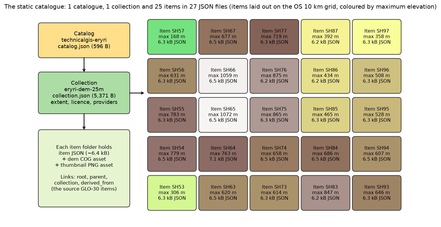
- pystac builds the Catalog → Collection → Item tree, and rio-stac reads each COG to fill in the geometry, projection and raster statistics. 25 items took 0.64 s to build and 0.02 s to save as 27 JSON files (165.6 kB).
- validate_all() checks every object against the official JSON schemas, including extension schemas. A missing start_datetime or a proj:shape written as a string fails with a precise message.
- A static catalogue is just files: any web server or bucket can host it, but there is no search. Finding all 25 items over HTTP took 27 requests; pystac-client's search() refuses with DoesNotConformTo.
- A STAC API answers the same question in one or two requests: Earth Search returned the 4 GLO-30 source items in 2 requests, and Planetary Computer returned the same 4 IDs.
- Search results are links, not data. Reading Sentinel-2 true colour over 50 x 50 km at 100 m through the Earth Search hrefs fetched 2.55 MB from two COGs of 295 MB and 229 MB.
Before you start
- Part 1 of this series, or its 25 COG tiles (the script runs part 1 if they are missing)
- Python 3.10+ with pystac, pystac-client, rio-stac, jsonschema, rasterio, geopandas, matplotlib and requests
- Basic GeoPandas: GeoDataFrames, intersects and attribute filters
Short answer: to create a STAC catalogue in Python, make one pystac.Item per file (rio-stac’s create_stac_item(path, with_proj=True, with_raster=True) fills in the geometry, projection and band statistics from a COG), add the items to a pystac.Collection, add the collection to a pystac.Catalog, then call catalog.normalize_hrefs("stac"), catalog.validate_all() and catalog.save(catalog_type=pystac.CatalogType.SELF_CONTAINED). The result is a folder of JSON files that you can host anywhere. To search a public STAC API instead, use pystac-client: Client.open(url).search(collections=[...], bbox=[...], datetime="...").
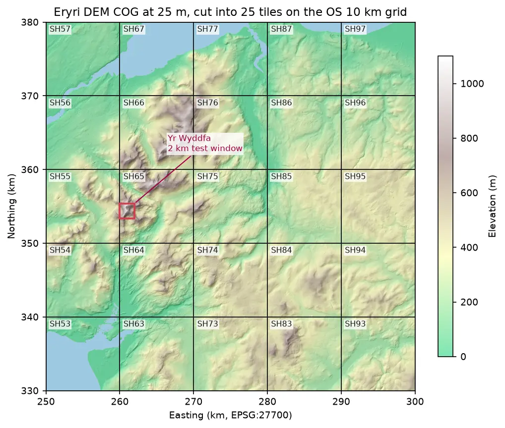
This is part 2 of the two-part series Cloud-native rasters in Python. In part 1 we mosaicked Copernicus DEM tiles from AWS into a Cloud Optimised GeoTIFF of Eryri and cut it into 25 COG tiles on the Ordnance Survey 10 km grid. Now we describe those tiles with STAC, the metadata standard behind Earth Search, Planetary Computer and most public satellite archives, so that people and programs can find them by place, time and properties.
You will learn how to:
- build a Catalog → Collection → Item tree with pystac, with items made by rio-stac;
- use the projection and raster extensions, and date ranges for products made from several years of data;
- validate every object against the STAC JSON schemas, and read the errors;
- read the catalogue back and query it by point, bounding box and property;
- serve it as static files, and see what that means for clients;
- search Earth Search and Planetary Computer with pystac-client, and read pixels through the results.
All outputs below are real results from stac_catalogue.py, run on 3 November 2026 on Windows 11 from the UK with Python 3.12.0, pystac 1.15.2, pystac-client 0.9.1, rio-stac 0.12.0, rasterio 1.5.2 (GDAL 3.12.2) and GeoPandas 1.2.0.
Set up
pip install pystac==1.15.2 pystac-client==0.9.1 rio-stac==0.12.0 jsonschema==4.26.0 rasterio==1.5.2 rio-cogeo==7.0.4 geopandas==1.2.0 shapely==2.2.0 matplotlib==3.11.2 requests==2.34.2pystac 1.15 writes STAC 1.1.0. jsonschema is needed only for validation, and rio-cogeo only if the script has to rebuild part 1’s tiles.
Step 1: build the catalogue
A STAC catalogue is a tree of three object types:
- Items describe one place and time each, here one 10 km tile, and point to its files (assets).
- A Collection groups items that share a licence, providers and extent, and summarises them.
- A Catalog is the root, which links to collections or other catalogues.
rio-stac opens a raster and builds an item from it: the footprint in longitude and latitude, the bounding box, the projection fields and per-band statistics.
import pystacfrom rio_stac import create_stac_item
ACQUIRED = (datetime(2011, 1, 1, tzinfo=timezone.utc), datetime(2015, 12, 31, 23, 59, 59, tzinfo=timezone.utc))
item = create_stac_item(    str(path),                                  # e.g. ../cloud-optimised-geotiff-python/output/tiles/SH65.tif    id=f"eryri-dem-25m-{name}",    input_datetime=ACQUIRED[0],    asset_name="dem",    asset_roles=["data"],    asset_media_type=pystac.MediaType.COG,    with_proj=True,    with_raster=True,    geom_densify_pts=10,    geom_precision=6,    properties={"os:grid_square": name, "processing:software": {"rasterio": rasterio.__version__}},)# A DEM built from 2011-2015 acquisitions has a date range, not an instant.item.datetime = Noneitem.common_metadata.start_datetime, item.common_metadata.end_datetime = ACQUIREDitem.common_metadata.created = PROCESSED
Three details are worth copying:
- Dates. Every STAC item must have a time. GLO-30 was built from TanDEM-X acquisitions between 2011 and 2015, so we set
datetimetonulland givestart_datetimeandend_datetimeinstead, which the specification allows.createdrecords when we made the file. - Densified footprints. Our tiles are squares in British National Grid, so in longitude and latitude their edges are slightly curved.
geom_densify_pts=10adds points along each edge before reprojecting. - Lineage. Each item gets
derived_fromlinks to the Earth Search items for the GLO-30 tiles that it came from. Step 5 checks them.
rio-stac 0.12 still writes version 1.1 of the projection extension, with proj:epsg: 27700. Version 2.0, which Earth Search uses, replaced it with proj:code: "EPSG:27700", so the script upgrades each item. It also recomputes valid_percent, which rio-stac 0.12 reported as 0.000625 instead of 100:
item.properties["proj:code"] = f"EPSG:{item.properties.pop('proj:epsg')}"item.stac_extensions = [u.replace("projection/v1.1.0", "projection/v2.0.0") for u in item.stac_extensions]item.assets["dem"].extra_fields["raster:bands"][0]["statistics"]["valid_percent"] = \ round(100 * float(np.isfinite(full).mean()), 2)item.add_asset("thumbnail", pystac.Asset(href=str(thumb), media_type=pystac.MediaType.PNG, roles=["thumbnail"], title="Hillshaded preview, 100 x 100 px"))Then the collection and the catalogue:
collection = pystac.Collection(    id="eryri-dem-25m",    title="Eryri DEM, 25 m, British National Grid",    description="Copernicus DEM GLO-30 over a 50 x 50 km area of Eryri (Snowdonia), ...",    extent=pystac.Extent(pystac.SpatialExtent([union_of_item_bboxes]),                         pystac.TemporalExtent([[ACQUIRED[0], ACQUIRED[1]]])),    license="other",    providers=[pystac.Provider("European Space Agency / Airbus", roles=[pystac.ProviderRole.LICENSOR,                                                                     pystac.ProviderRole.PRODUCER]),               pystac.Provider("TechnicalGIS", roles=[pystac.ProviderRole.PROCESSOR, pystac.ProviderRole.HOST])],)collection.add_link(pystac.Link("license", COPERNICUS_DEM_LICENCE_PDF, media_type="application/pdf"))collection.add_items(items)collection.summaries.add("os:grid_square", sorted(i.properties["os:grid_square"] for i in items))
catalog = pystac.Catalog(id="technicalgis-eryri", description="A static STAC catalogue built for ...")catalog.add_child(collection)catalog.normalize_hrefs("output/stac")# (the script copies each COG and thumbnail into its item's folder here)catalog.make_all_asset_hrefs_relative()catalog.save(catalog_type=pystac.CatalogType.SELF_CONTAINED)
license="other" plus a license link is how STAC records a licence that has no SPDX identifier, as with the Copernicus DEM licence. normalize_hrefs lays the tree out in pystac’s standard folders. A self-contained catalogue uses only relative links and has no self links, so the folder can be copied, zipped or uploaded anywhere. Call make_all_asset_hrefs_relative() before saving: without it, the asset hrefs kept the absolute Windows paths of the copies, and the catalogue broke as soon as it was served over HTTP.
pystac 1.15.2, STAC version 1.1.0; built 25 items in 0.64 s, saved in 0.02 s27 JSON files (165.6 kB) and 50 asset files (13.18 MB) stac/catalog.json 596 bytes stac/eryri-dem-25m/collection.json 5,371 bytes stac/eryri-dem-25m/eryri-dem-25m-SH53/eryri-dem-25m-SH53.json 6,273 bytes stac/eryri-dem-25m/eryri-dem-25m-SH97/eryri-dem-25m-SH97.json 6,277 bytesHere is the item for SH65, the square that contains Yr Wyddfa, with the long proj:geometry and proj:projjson fields left out:
{"stac_extensions": ["https://stac-extensions.github.io/projection/v2.0.0/schema.json", "https://stac-extensions.github.io/raster/v1.1.0/schema.json"], "bbox": [-4.093381, 53.028914, -3.940011, 53.121278], "properties": {"os:grid_square": "SH65", "processing:software": {"rasterio": "1.5.2"}, "proj:bbox": [260000.0, 350000.0, 270000.0, 360000.0], "proj:shape": [400, 400], "proj:transform": [25.0, 0.0, 260000.0, 0.0, -25.0, 360000.0, 0.0, 0.0, 1.0], "start_datetime": "2011-01-01T00:00:00Z", "end_datetime": "2015-12-31T23:59:59Z", "created": "2026-11-03T00:00:00Z", "title": "Eryri DEM 25 m, OS square SH65", "proj:code": "EPSG:27700", "datetime": null}, "assets.dem": {"href": "./SH65.tif", "type": "image/tiff; application=geotiff; profile=cloud-optimized", "roles": ["data"]}, "dem band statistics": {"mean": 439.93389892578125, "minimum": 53.640750885009766, "maximum": 1071.8411865234375, "stddev": 202.7344970703125, "valid_percent": 100.0}, "links (rel)": ["derived_from", "derived_from", "root", "collection", "parent"]}The proj: fields let a client place the pixels in British National Grid without opening the COG, and the band statistics let it filter by elevation. The asset href ./SH65.tif is relative to the item’s JSON file.
Step 2: validate against the STAC schemas
Every STAC object names its schemas: the core schema for its type and version, plus one per extension in stac_extensions. validate_all() walks the tree and checks every object against all of them:
n_valid = catalog.validate_all()validate_all: 25 items valid (plus the catalogue and collection); first pass 0.40 s (fetches the schemas), second pass 0.23 s (schemas cached)The first pass downloads the schemas from schemas.stacspec.org and stac-extensions.github.io; pystac caches them for the rest of the session. To see what a failure looks like, we break two copies of the SH65 item and validate each with pystac.validation.validate_dict. The STACValidationError carries the underlying jsonschema errors, and jsonschema.exceptions.best_match picks the most useful one:
no_start = json.loads(json.dumps(sh65))no_start["properties"].pop("start_datetime") # datetime is null, so start and end become mandatorybad_shape = json.loads(json.dumps(sh65))bad_shape["properties"]["proj:shape"] = "400 x 400" # must be an array of integersfor label, doc in [("start_datetime removed", no_start), ("proj:shape as a string", bad_shape)]: try: pystac.validation.validate_dict(doc) except pystac.STACValidationError as err: best = jsonschema.exceptions.best_match(err.source) print(label, best.message, "/".join(map(str, best.absolute_path))) start_datetime removed: STACValidationError schema: https://schemas.stacspec.org/v1.1.0/item-spec/json-schema/item.json reason: 'start_datetime' is a required property (at properties) proj:shape as a string: STACValidationError schema: https://stac-extensions.github.io/projection/v2.0.0/schema.json reason: '400 x 400' is not of type 'array' (at properties/proj:shape)The first error comes from the core item schema, which requires start_datetime and end_datetime whenever datetime is null. The second comes from the projection extension’s schema. Validation only checks structure and types: it would not notice a bounding box in the wrong place, so check footprints visually as well (Figure 2).
Step 3: read it back and query it
pystac.Catalog.from_file reads the root and follows links lazily. Here we load all items into a GeoDataFrame, with the band statistics as columns:
cat = pystac.Catalog.from_file("output/stac/catalog.json")local_items = list(cat.get_items(recursive=True))rows = []for it in local_items:    band = it.assets["dem"].extra_fields["raster:bands"][0]    rows.append({"id": it.id, "square": it.properties["os:grid_square"], "max_m": band["statistics"]["maximum"],                 "href": it.assets["dem"].get_absolute_href(), "geometry": shape(it.geometry)})gdf = gpd.GeoDataFrame(rows, crs="EPSG:4326")
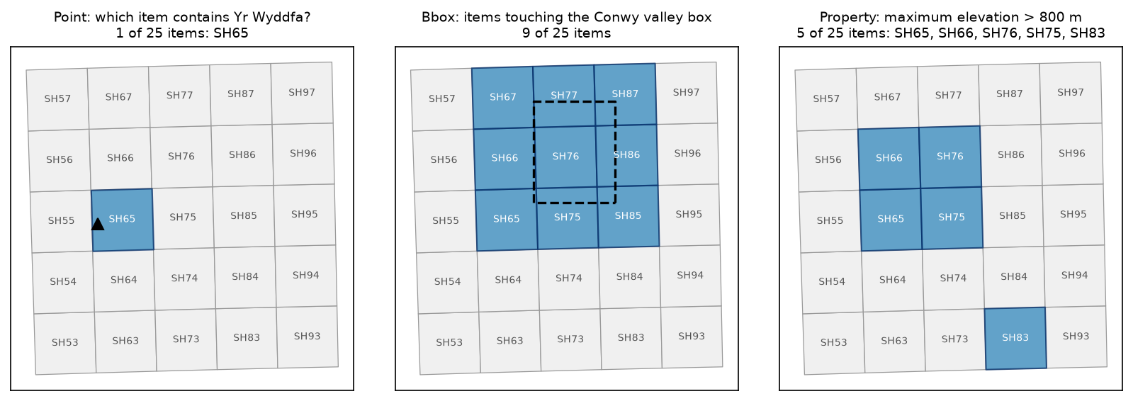
proj = ProjectionExtension.ext(local_items[0])      # typed access to the proj: fieldsq_point = gdf[gdf.intersects(Point(-4.0763, 53.0685))]q_bbox = gdf[gdf.intersects(box(-3.95, 53.10, -3.75, 53.25))]q_high = gdf[gdf.max_m > 800].sort_values("max_m", ascending=False)
read 25 items from disk in 0.014 s; projection extension on eryri-dem-25m-SH53: code EPSG:27700, shape [400, 400], bbox [250000.0, 330000.0, 260000.0, 340000.0]point query (Yr Wyddfa (-4.0763, 53.0685)): ['SH65']bbox query (-3.95, 53.10, -3.75, 53.25): 9 items ['SH65', 'SH66', 'SH67', 'SH75', 'SH76', 'SH77', 'SH85', 'SH86', 'SH87']property query (maximum elevation > 800 m): 5 itemssquare min_m mean_m max_m SH65 53.6 439.9 1071.8 SH66 33.0 492.9 1059.2 SH76 1.0 312.6 875.1 SH75 8.2 272.0 865.0 SH83 158.5 363.4 846.5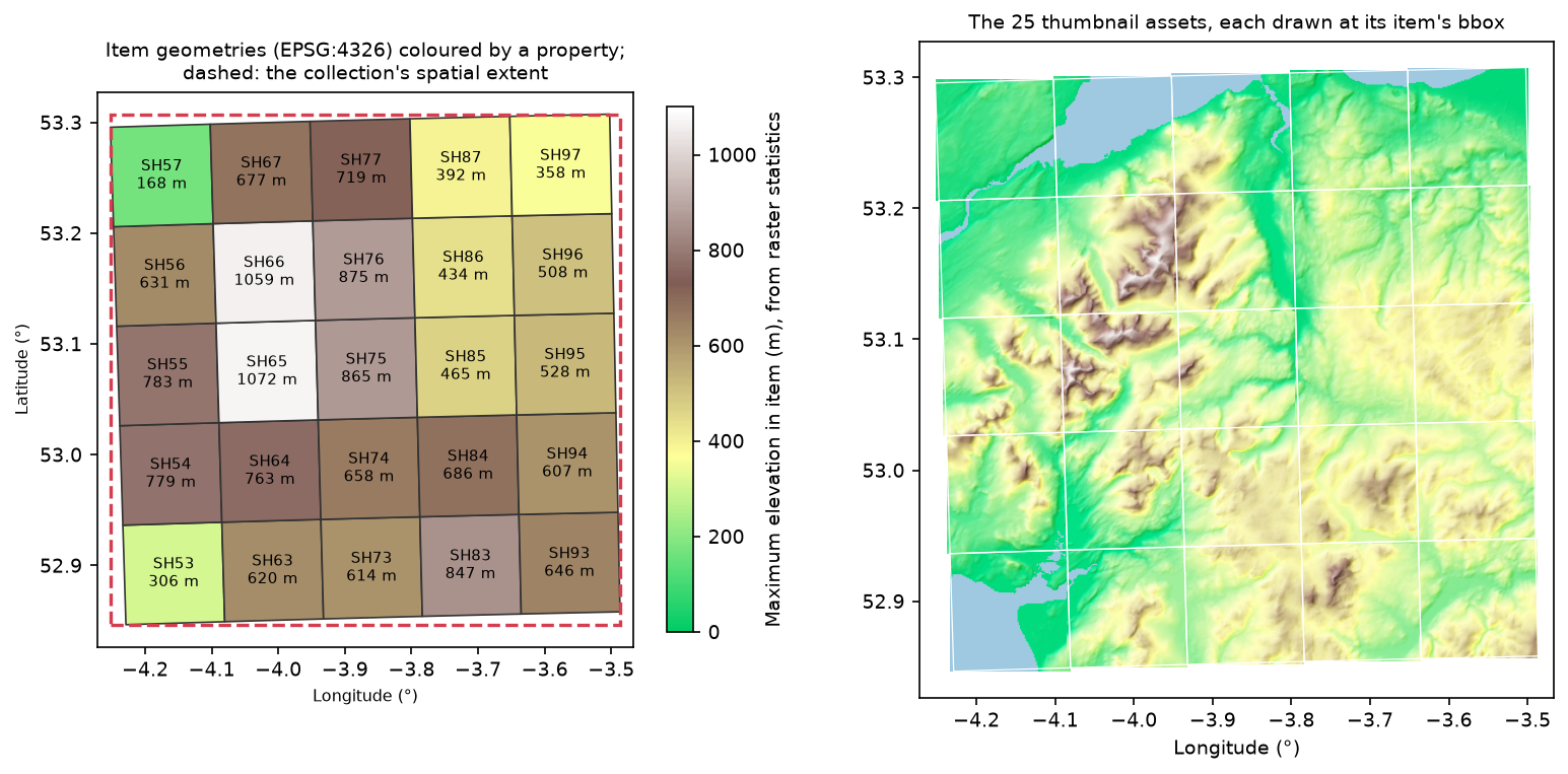
For 25 items, a GeoDataFrame is the simplest search engine. For thousands, write the items to a GeoParquet file with the stac-geoparquet package and query it with DuckDB or GeoPandas, as in GeoParquet and DuckDB with Overture Maps.
Step 4: serve it as static files
A self-contained catalogue works from any web server or bucket. The script serves output/stac/ on localhost with a small http.server subclass that supports Range requests and counts every GET, then crawls it as a remote client would:
remote_cat = pystac.Catalog.from_file(f"{base}/catalog.json")crawled = list(remote_cat.get_items(recursive=True))
one = pystac.Item.from_file(f"{base}/eryri-dem-25m/eryri-dem-25m-SH65/eryri-dem-25m-SH65.json")with rasterio.open(one.assets["dem"].get_absolute_href()) as src:    win = src.read(1, window=rasterio.windows.from_bounds(260_000, 353_000, 262_000, 355_000, src.transform))
static_client = Client.open(f"{base}/catalog.json")static_client.search(bbox=[-4.1, 53.0, -4.0, 53.1]).item_collection()
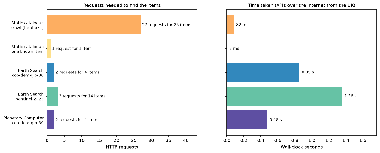
crawl all items: 25 items, 27 GET requests, 165.6 kB of JSON, 0.08 s first requests: ['/catalog.json', '/eryri-dem-25m/collection.json', '/eryri-dem-25m/eryri-dem-25m-SH53/eryri-dem-25m-SH53.json']fetch one item you already know: 1 request, 6.5 kB, 2 mspystac-client search on the static catalogue: DoesNotConformTo: Server does not conform to ITEM_SEARCH, There is no fallback option available for search.read a 2 x 2 km window of SH65 through its asset href: 3 range requests, 285.9 kB of a 537.8 kB file, max 1071.8 m, 8 ms- Crawling costs one request per object. A client must read the catalogue, the collection and every item before it can answer “which items touch this box?”. That is 27 requests here, and millions for an archive the size of Sentinel-2.
- Known items are cheap. If you know the path, an item is one request.
- pystac-client refuses to search. A static catalogue declares no API conformance classes, so
search()raisesDoesNotConformTorather than crawling silently. - The asset hrefs work over HTTP. pystac resolved
./SH65.tifagainst the item’s URL, and rasterio read a 2 x 2 km window with three range requests, as in part 1.
For browsing, point STAC Browser at the hosted catalog.json. For search, load the items into a STAC API such as stac-fastapi with pgstac.
Step 5: search public STAC APIs with pystac-client
A STAC API adds a /search endpoint on top of the same JSON objects. Earth Search, run by Element 84, catalogues AWS Open Data, including the GLO-30 tiles that part 1 read, so we can ask it for our sources:
from pystac_client import Client
es = Client.open("https://earth-search.aws.element84.com/v1")es_dem = list(es.search(collections=["cop-dem-glo-30"], bbox=aoi_bbox).items())
s2 = list(es.search(collections=["sentinel-2-l2a"], intersects=box(*aoi_bbox).__geo_interface__,                    datetime="2026-05-01/2026-09-30", query={"eo:cloud_cover": {"lt": 10}},                    sortby=[{"field": "properties.eo:cloud_cover", "direction": "asc"}], max_items=100).items())
pc = Client.open("https://planetarycomputer.microsoft.com/api/stac/v1")pc_items = list(pc.search(collections=["cop-dem-glo-30"], bbox=aoi_bbox).items())
The script counts requests with a requests response hook on each client’s session:
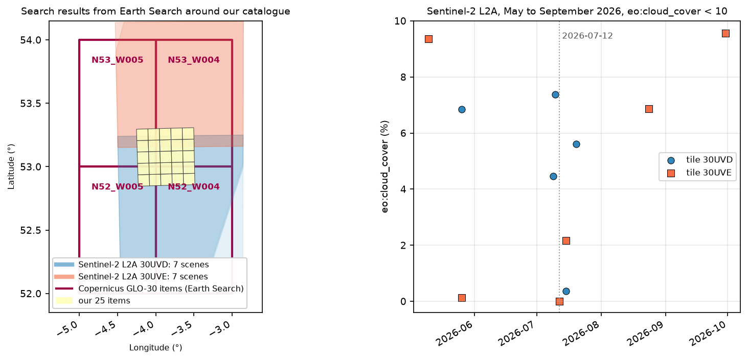
Earth Search: opened landing page in 0.39 s; 9 collectionscop-dem-glo-30 in bbox [-4.2521, 52.8466, -3.4867, 53.3075]: 4 items, 2 POST request(s), 0.85 s Copernicus_DSM_COG_10_N53_00_W005_00_DEM datetime 2021-04-22 s3://copernicus-dem-30m/Copernicus_DSM_COG_10_N53_00_W005_00_DEM/Copernicus_DSM_COG_10_N53_00_W005_00_DEM.tif Copernicus_DSM_COG_10_N53_00_W004_00_DEM datetime 2021-04-22 s3://copernicus-dem-30m/Copernicus_DSM_COG_10_N53_00_W004_00_DEM/Copernicus_DSM_COG_10_N53_00_W004_00_DEM.tif Copernicus_DSM_COG_10_N52_00_W005_00_DEM datetime 2021-04-22 s3://copernicus-dem-30m/Copernicus_DSM_COG_10_N52_00_W005_00_DEM/Copernicus_DSM_COG_10_N52_00_W005_00_DEM.tif Copernicus_DSM_COG_10_N52_00_W004_00_DEM datetime 2021-04-22 s3://copernicus-dem-30m/Copernicus_DSM_COG_10_N52_00_W004_00_DEM/Copernicus_DSM_COG_10_N52_00_W004_00_DEM.tifour derived_from links point at the same 4 items: Truesentinel-2-l2a, May-Sep 2026, cloud < 10%: 14 items, 3 request(s), 1.36 s id date mgrs cloud_%S2A_30UVE_20260510_0_L2A 2026-05-10 30UVE 9.355050S2B_30UVD_20260526_0_L2A 2026-05-26 30UVD 6.851021S2B_30UVE_20260526_0_L2A 2026-05-26 30UVE 0.121609S2A_30UVD_20260709_0_L2A 2026-07-09 30UVD 4.464607S2C_30UVD_20260710_0_L2A 2026-07-10 30UVD 7.375222S2B_30UVD_20260712_0_L2A 2026-07-12 30UVD 0.000561S2A_30UVD_20260712_1_L2A 2026-07-12 30UVD 0.000645S2B_30UVE_20260712_0_L2A 2026-07-12 30UVE 0.007792S2A_30UVE_20260712_1_L2A 2026-07-12 30UVE 0.008869S2B_30UVD_20260715_0_L2A 2026-07-15 30UVD 0.367485S2B_30UVE_20260715_0_L2A 2026-07-15 30UVE 2.161486S2C_30UVD_20260720_0_L2A 2026-07-20 30UVD 5.617763S2B_30UVE_20260824_0_L2A 2026-08-24 30UVE 6.859924S2B_30UVE_20260930_0_L2A 2026-09-30 30UVE 9.563044Planetary Computer cop-dem-glo-30: 4 items, 2 requests (including the landing page), 0.48 s same item IDs as Earth Search: True example href: https://elevationeuwest.blob.core.windows.net/copernicus-dem/COP30_hh/Copernicus_DSM_COG_10_N53_00_W005_00_DEM.tifWhat the comparison shows:
- Search is one round trip. Each API answered a spatial search in a couple of requests and well under 1.5 s from the UK, wherever the archive is stored. pystac-client follows the API’s
nextlinks for paging, so you never handle pages yourself. - The same data, catalogued twice. Both APIs return the same four GLO-30 item IDs, but the asset hrefs differ: an
s3://URL on AWS, and an Azure Blob URL on Planetary Computer, which needs a short-lived SAS token before you can read it (theplanetary-computerpackage’ssign()adds one). Ourderived_fromlinks match the Earth Search IDs exactly. - Check what
datetimemeans. Earth Search dates the GLO-30 items 2021-04-22, the publication date, although the radar data is from 2011–2015. Our items use a date range instead. When you search by time, read the collection’s description to learn which date it uses. - Expect more than one item per tile and date. 2026-07-12 has two items for each Sentinel-2 tile, with IDs ending
_0and_1and different satellite prefixes. The script keeps the least cloudy item for each tile.
Step 6: read pixels through the hrefs
A search returns metadata. To get pixels, open the asset hrefs. From our own catalogue, we merge the five items that the property query found, straight from their hrefs:
mosaic, mosaic_tf = merge(list(q_high.href), nodata=np.nan) # NaN where no item covers the bounding boxmerged the 5 items with maximum > 800 m from local hrefs: 1200 x 1600 px in 0.03 s; max 1071.8 m; 58% of the box has no itemFrom Earth Search, we take the clearest date that covers both Sentinel-2 tiles, keep one item per tile, and read the visual (true colour) asset of each. Each is a 10980 x 10980 px COG with overviews, so we open overview level 2 (1/8, 80 m) and warp it to our 100 m British National Grid with a WarpedVRT:
for it in best: href = it.assets["visual"].href # Overview level 2 is the 1/8 overview (80 m), the closest one finer than our 100 m target. with rasterio.open(href, overview_level=2) as src, \ WarpedVRT(src, crs="EPSG:27700", transform=s2_tf, width=s2_shape[1], height=s2_shape[0], resampling=Resampling.average) as vrt: part = vrt.read() fill = (rgb.sum(axis=0) == 0) & (part.sum(axis=0) > 0) rgb[:, fill] = part[:, fill]clearest date covering both MGRS tiles: 2026-07-12; 4 items, using S2B_30UVD_20260712_0_L2A, S2B_30UVE_20260712_0_L2A S2B_30UVD_20260712_0_L2A: visual asset 10980 x 10980 px at 10 m, overviews [2, 4, 8, 16], 295 MB S2B_30UVE_20260712_0_L2A: visual asset 10980 x 10980 px at 10 m, overviews [2, 4, 8, 16], 229 MBSentinel-2 true colour over the 50 x 50 km area at 100 m: 5 range requests, 2.55 MB, 4.4 s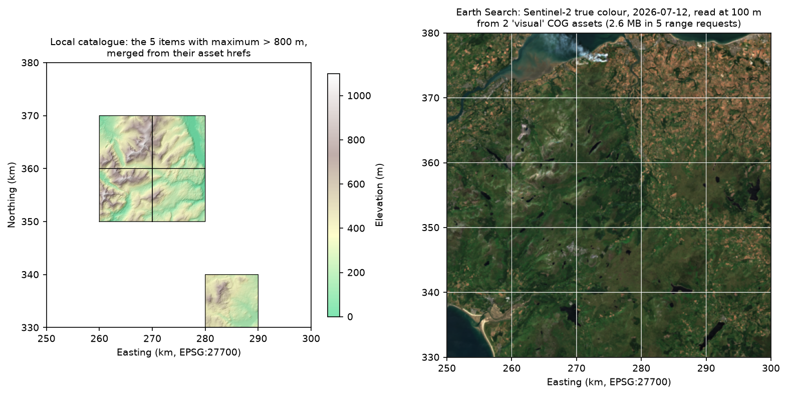
Our first attempt read the full-resolution assets and let GDAL resample: it fetched 231 MB and took 68 s. Opening the overview explicitly cut that by 99%. Whenever you read a large COG at low resolution, pick the overview yourself or check that your reader does.
Limitations and caveats
- rio-stac lags the extensions. Version 0.12 writes projection v1.1 and reports
valid_percentwrongly, so the script patches both. Check the output of any generator against the current extension schemas. - Validation is structural. Valid JSON can still describe the wrong footprint, date or licence. Plot the footprints and read a few items.
- Static catalogues don’t scale for search. Fine for tens or thousands of items you link to directly; for search over many items, use a STAC API or stac-geoparquet.
- API results change. Earth Search and Planetary Computer add and reprocess items, so the Sentinel-2 list and its cloud cover can differ when you run the script. The GLO-30 items are stable.
- Timings are from one connection. The API times depend on your network and the services’ load; the request counts are the stable figures.
Frequently asked questions
How do I create a STAC catalog in Python?
Install pystac, create a pystac.Item for each file (or let rio-stac’s create_stac_item build it from a raster), add the items to a pystac.Collection with an extent and licence, and add that to a pystac.Catalog. Then call normalize_hrefs(root_folder), validate_all() and save(catalog_type=pystac.CatalogType.SELF_CONTAINED). Here that produced 27 JSON files for 25 COGs in under a second.
What is the difference between pystac and pystac-client?
pystac reads, writes and validates STAC objects, whether they are files on disk or JSON on a web server. pystac-client talks to STAC APIs: it checks what an API supports, sends /search requests with your bbox, time and property filters, and follows the paging links. It returns pystac objects, so the two work together.
What is the difference between a static STAC catalogue and a STAC API?
A static catalogue is JSON files linked to each other; you host it anywhere, but clients must crawl it to find items (27 requests for our 25). A STAC API is a service with a /search endpoint, which answers spatial, temporal and property queries in one request. Many projects publish a static catalogue first and load it into an API when it grows.
How do I validate a STAC catalog?
Call catalog.validate_all() in pystac, which needs jsonschema installed. It checks every object against the core schemas and every extension schema it lists, and raises STACValidationError on the first failure. Use jsonschema.exceptions.best_match(err.source) for the most specific message. The stac-validator command-line tool does the same outside Python.
Can I search Earth Search or Planetary Computer without an account?
Yes. Both STAC APIs are open for searching without keys. Earth Search’s Sentinel-2 assets are public URLs. Planetary Computer’s assets need a free, short-lived SAS token, which the planetary-computer package adds with planetary_computer.sign(item), without an account.
Next steps
- Go back to part 1: Cloud Optimised GeoTIFFs in Python to change the area, resolution or COG settings, then rebuild this catalogue.
- Load Sentinel-2 search results into an xarray cube in NDVI time series with odc-stac.
- Search Sentinel-2 over a reservoir in Sentinel-2 and STAC: Lake Mead.
- Publish vector data the same cloud-native way with PMTiles vector tiles and MapLibre.
Data and licences
- Copernicus DEM GLO-30, via part 1. © DLR e.V. 2010–2014 and © Airbus Defence and Space GmbH 2014–2018, provided under COPERNICUS by the European Union and ESA; all rights reserved. The catalogue records this licence with
license: "other"and a link to the licence document. - Sentinel-2 L2A, via Earth Search. Contains modified Copernicus Sentinel data 2026, free and open under the Copernicus data policy.
- STAC metadata from Earth Search (Element 84) and the Microsoft Planetary Computer.
- Code:
stac_catalogue.py, tested with Python 3.12.0, pystac 1.15.2, pystac-client 0.9.1, rio-stac 0.12.0, jsonschema 4.26.0, rasterio 1.5.2 (GDAL 3.12.2), GeoPandas 1.2.0 and matplotlib 3.11.2. Pinned versions are inrequirements.txt.
Key terms
- STAC (SpatioTemporal Asset Catalog)
- A JSON specification for describing geospatial data so that it can be found by place and time. The core objects are Catalogs, Collections and Items; each Item points to files called assets.
- Static catalogue
- A STAC catalogue stored as plain JSON files linked to each other, which you can host on any web server or object store. Clients crawl it by following links; it has no search endpoint.
- STAC API
- A web service that serves STAC objects and adds endpoints such as /search, so clients can filter by bounding box, time and properties in one request. Earth Search and Planetary Computer are STAC APIs.
- Asset
- A file that an Item describes, such as a COG, a thumbnail or a metadata file, given by its href, media type and roles.
- STAC extension
- A versioned JSON schema that adds fields to STAC objects, such as projection (proj:code, proj:shape) or raster (band statistics). Items list the extensions they use in stac_extensions.
- pystac-client
- A Python client for STAC APIs that handles conformance checks, search parameters and paging, returning pystac objects.
Data for this tutorial
- Copernicus DEM GLO-30 · Source of the 25 COG tiles made in part 1
- Earth Search · Element 84's public STAC API for AWS Open Data, searched for cop-dem-glo-30 and sentinel-2-l2a
- Microsoft Planetary Computer STAC API · Searched for cop-dem-glo-30 for comparison
- STAC specification · Specification, extensions and the STAC Index of public catalogues
Licences and formats for each source are listed in the GIS data sources catalogue.